A Visual Guide to Gemma 4

A great start to a new job ;)

Translation - Korean

UPDATE - Added a section on Multi-Token Prediction (MTP) drafters for Gemma 4 😀

I’m beyond excited to announce the Gemma 4 family of models! It’s a big part of the reason why I joined Google DeepMind. Developing incredible research and sharing it with the world is something that even to this day, is ingrained in the culture of their research teams.

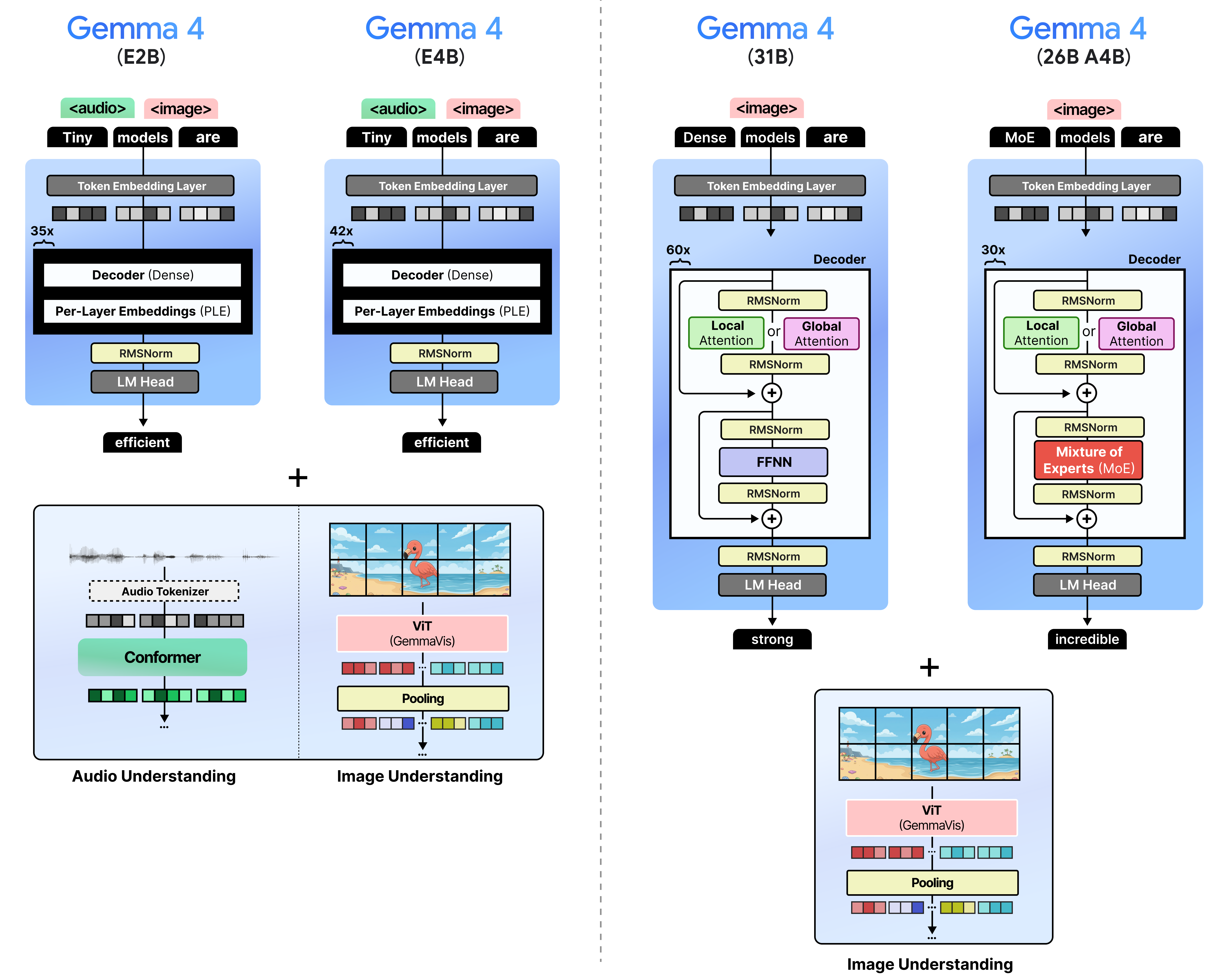
There are four models in the Gemma 4 family:

• Gemma 4 - E2B – A dense model with per-layer embeddings, which make them effectively 2 billion parameters

• Gemma 4 - E4B – A dense model with per-layer embeddings, which make them effectively 4 billion parameters

• Gemma 4 - 31B– A dense model with 31 billion parameters

• Gemma 4 - 26B A4B – A Mixture of Experts (MoE) model with 26 billion total parameters of which 4 billion are activated during inference.

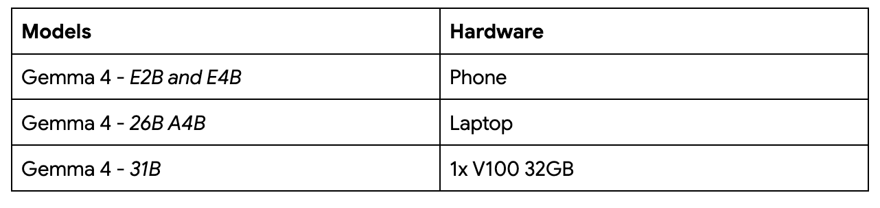
By having a broad range of model sizes, you can choose whichever model best suits your use case and whether it actually fits on your hardware:

There are two main architectures that are used across these models, namely dense and Mixture-of-Experts.

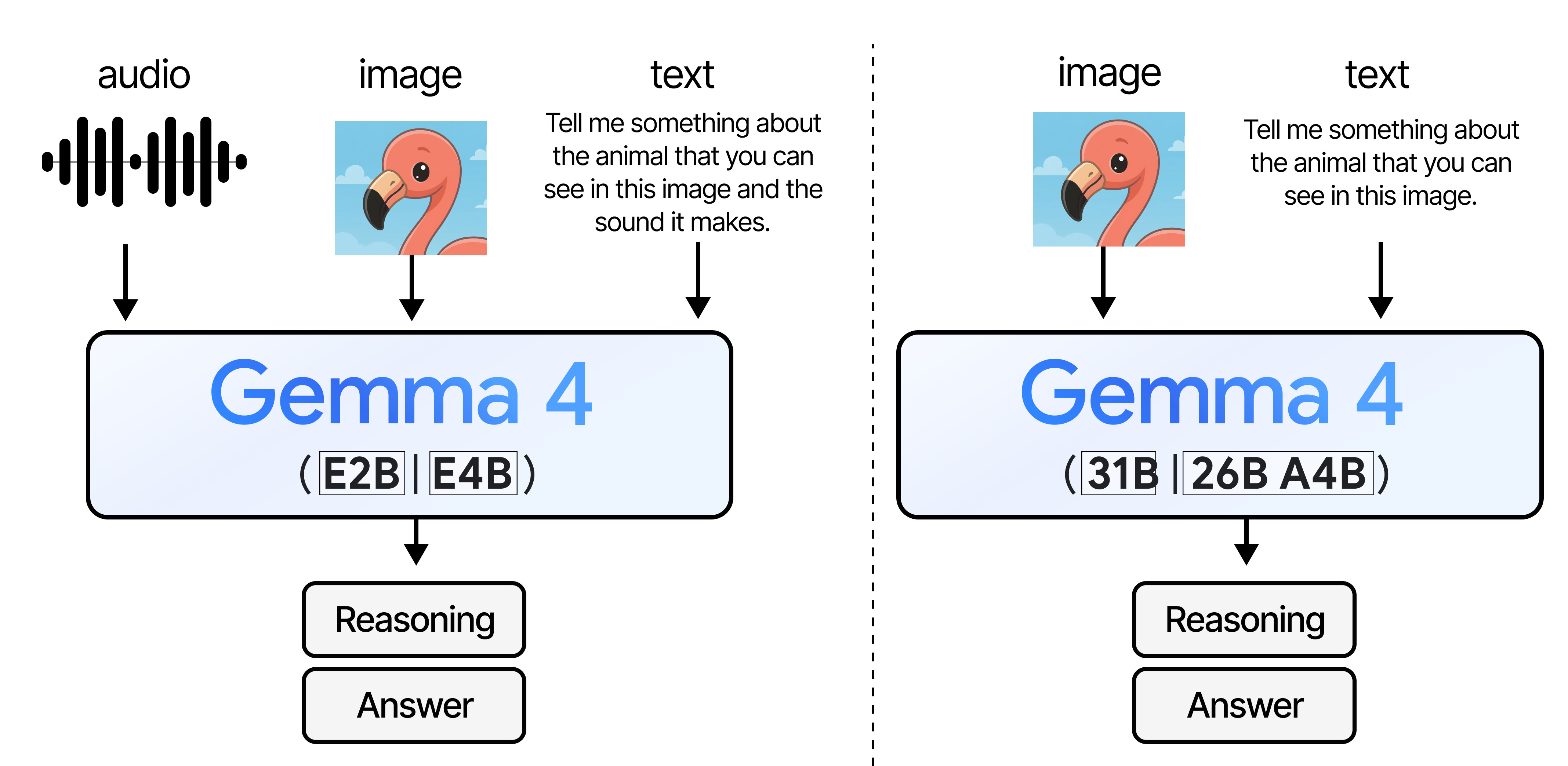
Aside from a wide range of sizes, all models are multimodal and can reason about input images. They were trained to handle many images of varying sizes (more on that later!).

I’m especially interested in trying out the small models a bit more since they not only support input images and text, but also audio.

There is A LOT to cover, but before I go into the specifics of the different sizes and architectures, let’s first explore what all models have in common!

👈 click on the stack of lines on the left to see a Table of Contents (ToC)

The Gemma 4 Architecture

The Gemma 4 architecture is in many ways like the Gemma 3 series of models, with some changes here and there. There are a number of things that were changed compared to Gemma 3 that relate to all model sizes:

• Interleaving Layers – Global attention is always the last layer

• K=V – The Keys are set to be equivalent to the Values only for the global attention

• p-RoPE – Low-frequency-pruned RoPE applied to the embeddings

Some of the models are a bit different than others (e.g., only small models use Per-Layer Embeddings). Before we go into the specifics of each model, let’s explore in more detail what they have in common.

Interleaving Layers

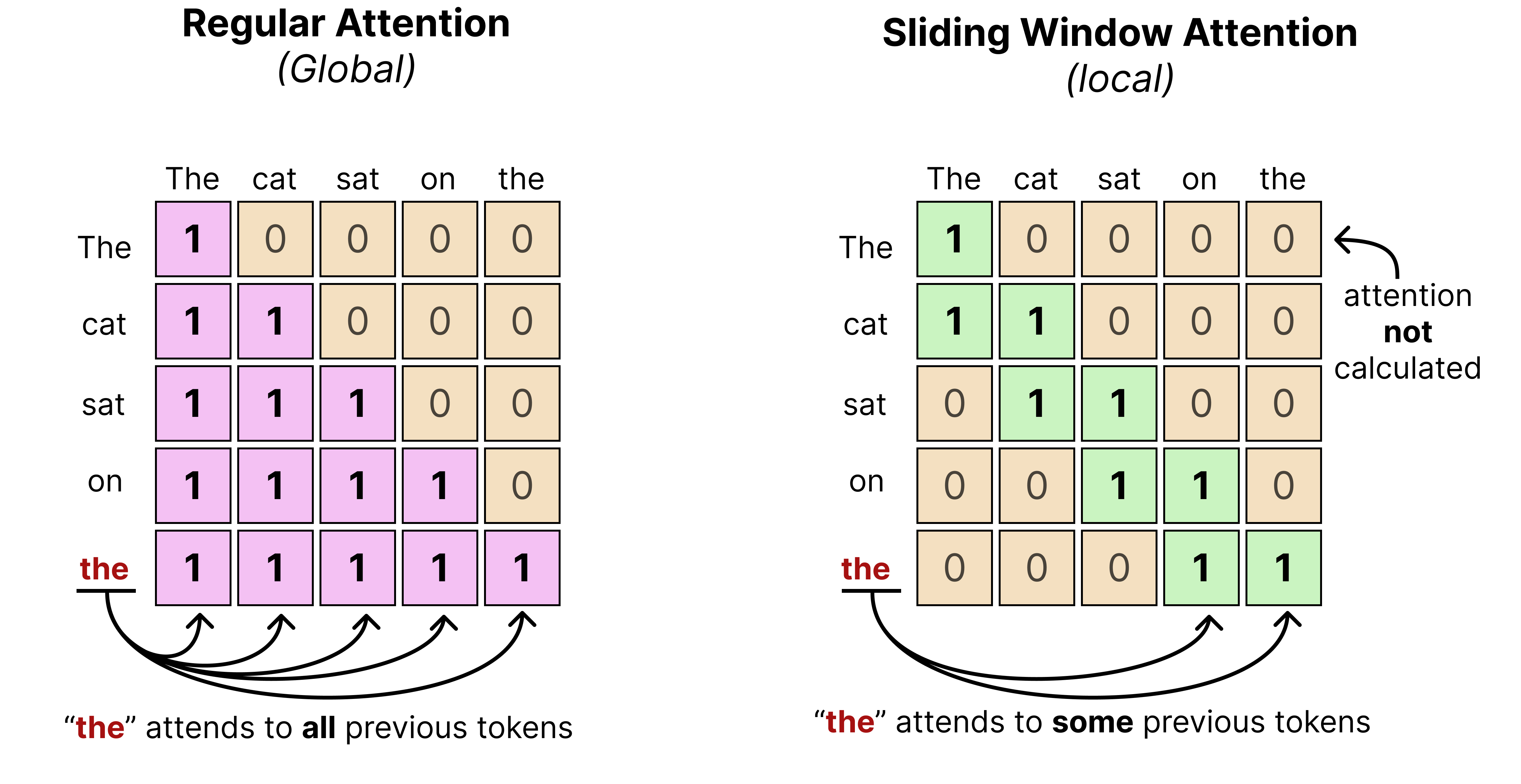
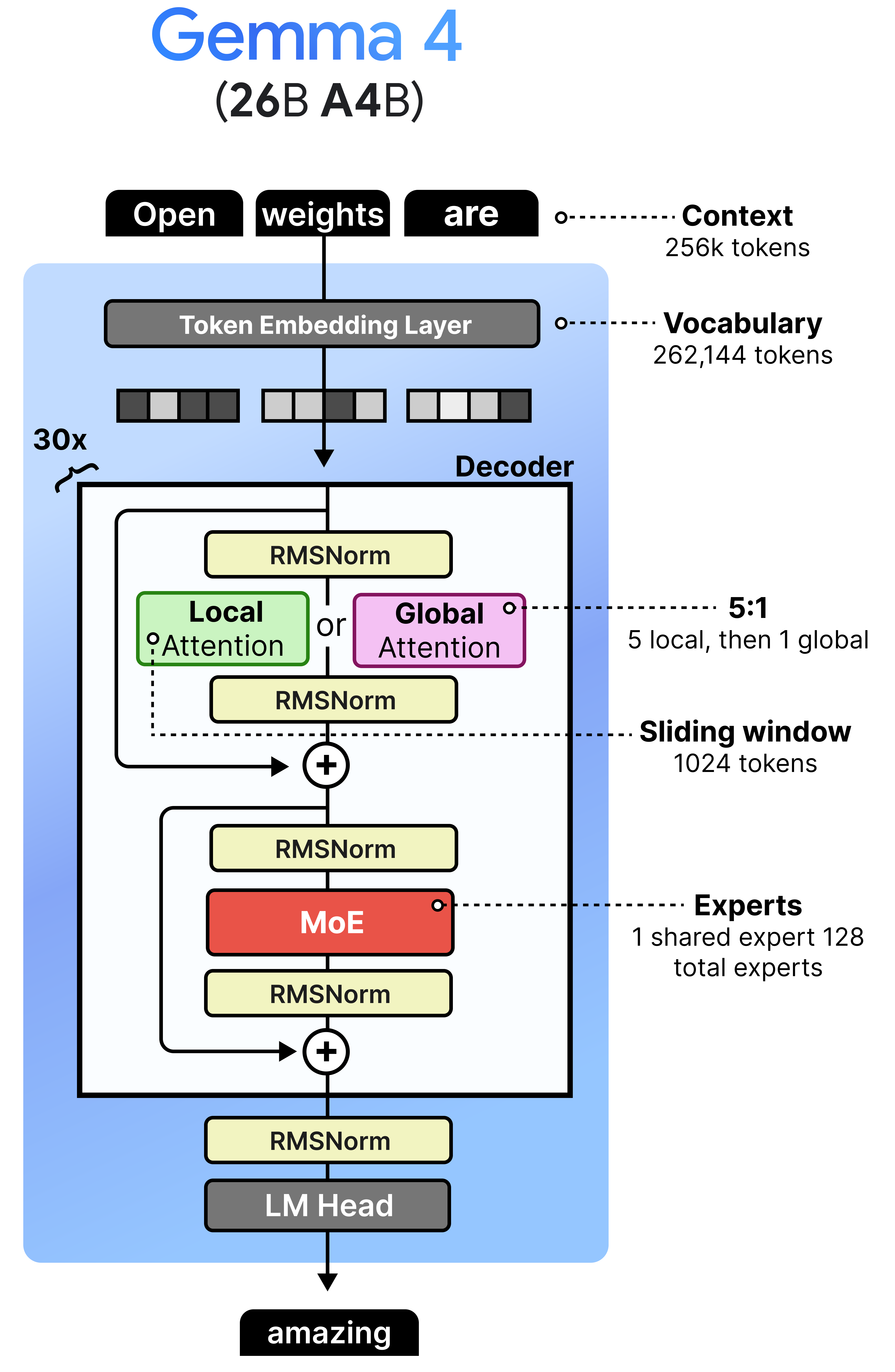
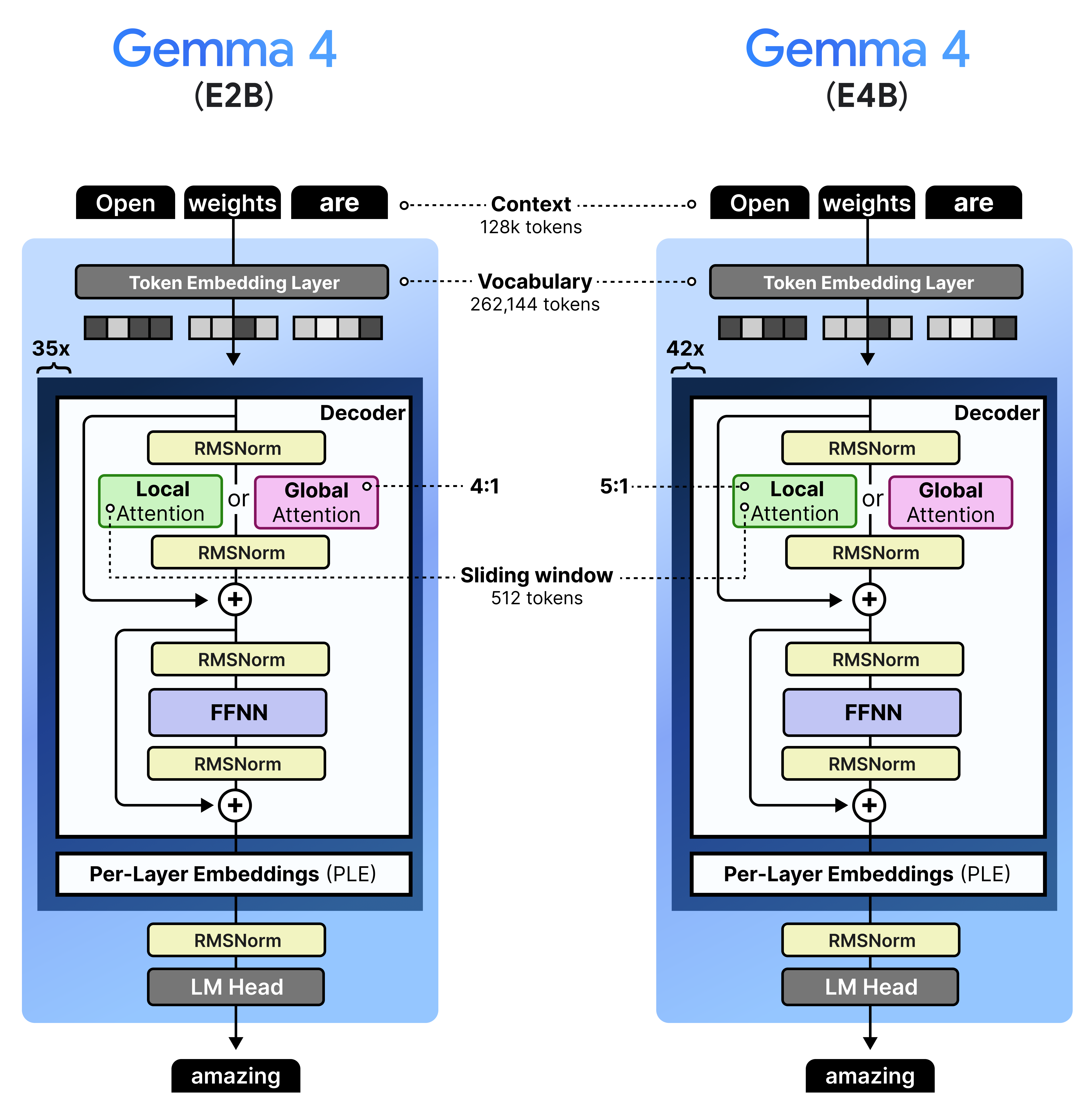
Like Gemma 3, Gemma 4 interleaves layers of local attention (also called “sliding window attention”) with global attention (which is regular or “full” attention).

Remember that in global attention, every token attends to all tokens that came before it. Sliding window attention, however, only attends to tokens within a certain limit. This significantly reduces the compute needed to calculate the full attention.

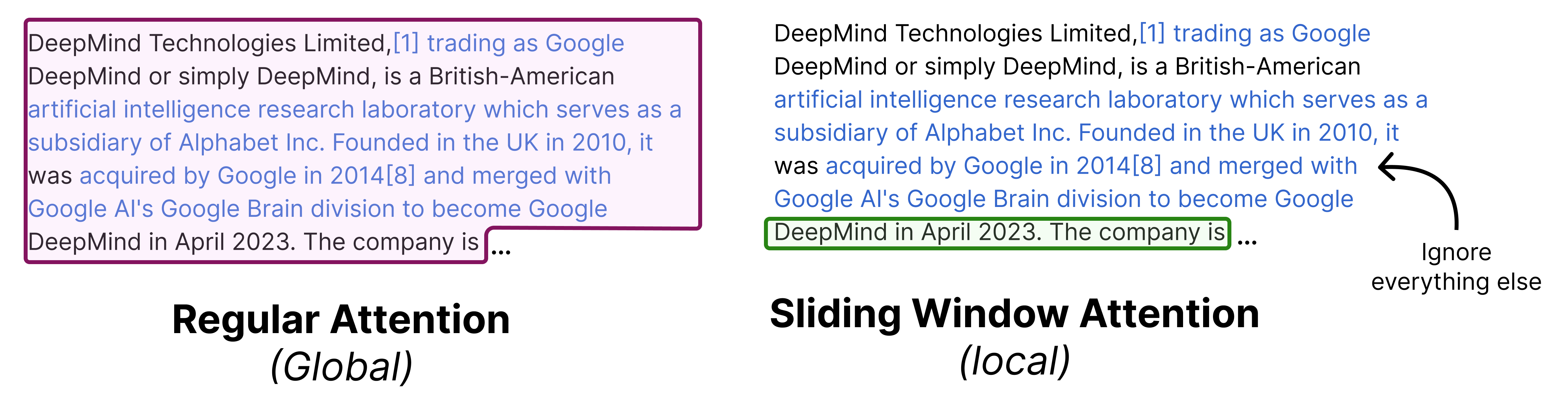
In practice, that means that when text is processed using a sliding window, it may only see a part of the entire sequence rather than the entire thing. The “sliding” then refers to the idea of continuously moving the sequence in view as the number of tokens are being generated.

You typically fix the number of tokens it can see previously. In the case of Gemma 4 models, the smaller models (E2B and E4B) have a sliding window of 512 tokens and the larger models (26B A4B and 31B) have a sliding window of 1024 tokens.

Let’s go through an example with a sliding window of 4 tokens to see what is happening at each token generation:

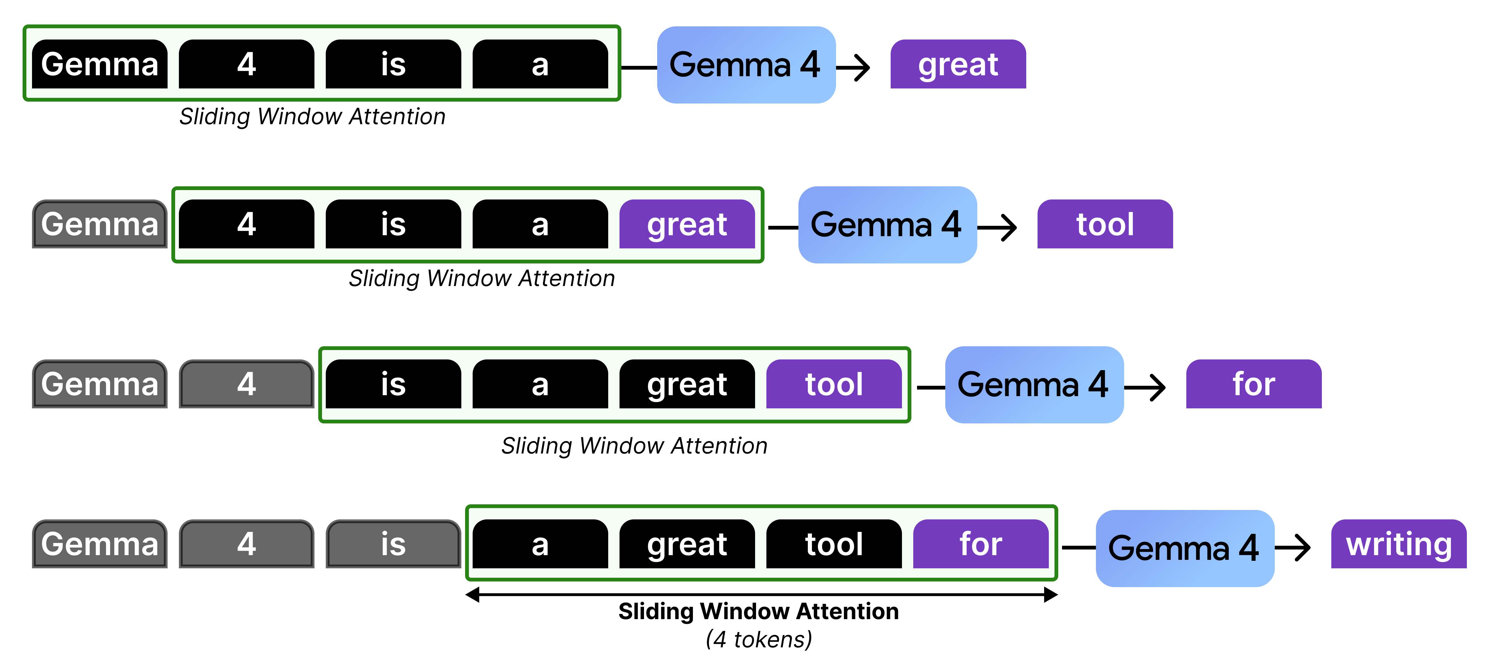
In our example, there is only attention given to the last four tokens which at some point in the generation starts to “ignore” the ones that came before that. However, it is actually not forgetting the representations that it calculated in the previous steps. The hidden states allow for the attention to be passed along the attention mechanism from previous layers and steps all the way to the current token.

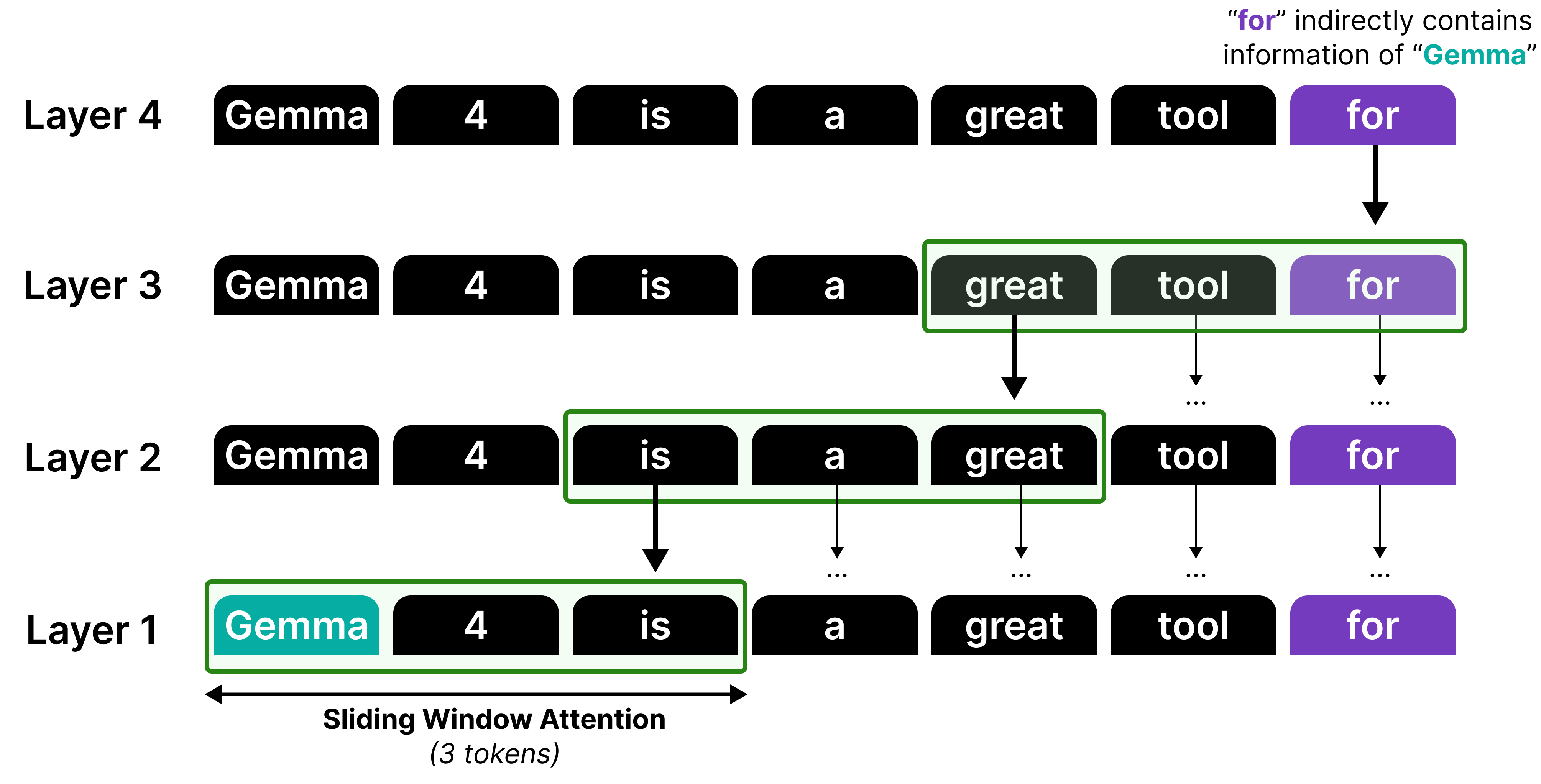
Although information can be propagated by stacking sliding windows, it is not a perfect recall or attention mechanism. Think of it like a game of telephone, information gets diluted each time it passes through another layer!

Therefore, much like in Gemma 3, local attention and global attention layers are interleaved such that the model does attend to the full sequence at times to better capture the global structure.

In Gemma 3, this interleaving was generally in a 4:1 pattern with 4 layers of local attention followed by a single layer of global attention. However, Gemma 3 - 4B for instance had 34 layers, which means its last layer used local attention rather than global attention. This was changed in the Gemma 4 models to make sure that the last layer is always global attention.

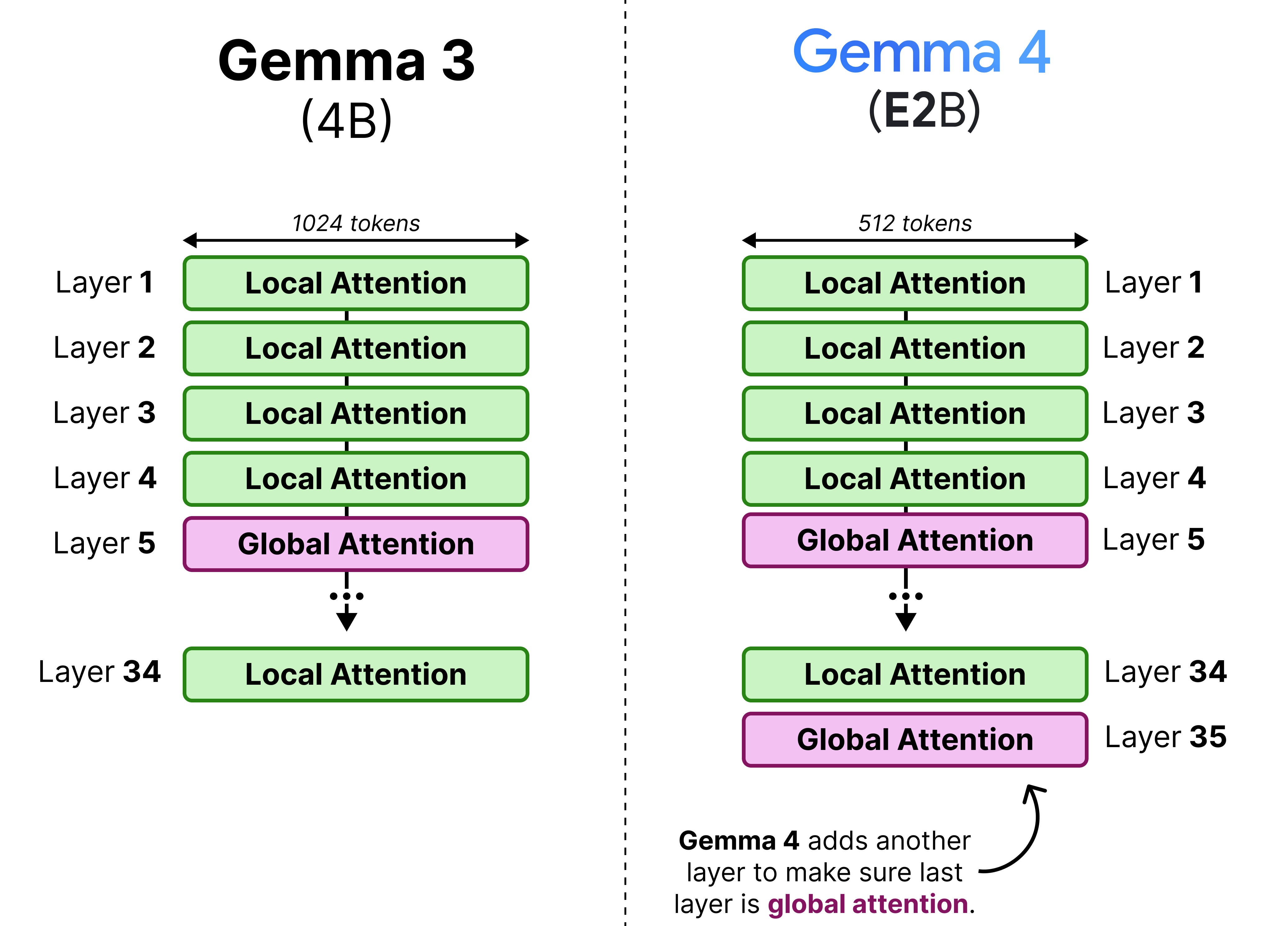
The 4:1 pattern, however, is only for the E2B as all other variants have a 5:1 pattern where they start with 5 layers of local attention followed by a single layer of global attention. We can visualize this pattern side-by-side to also demonstrate the depth of these models.

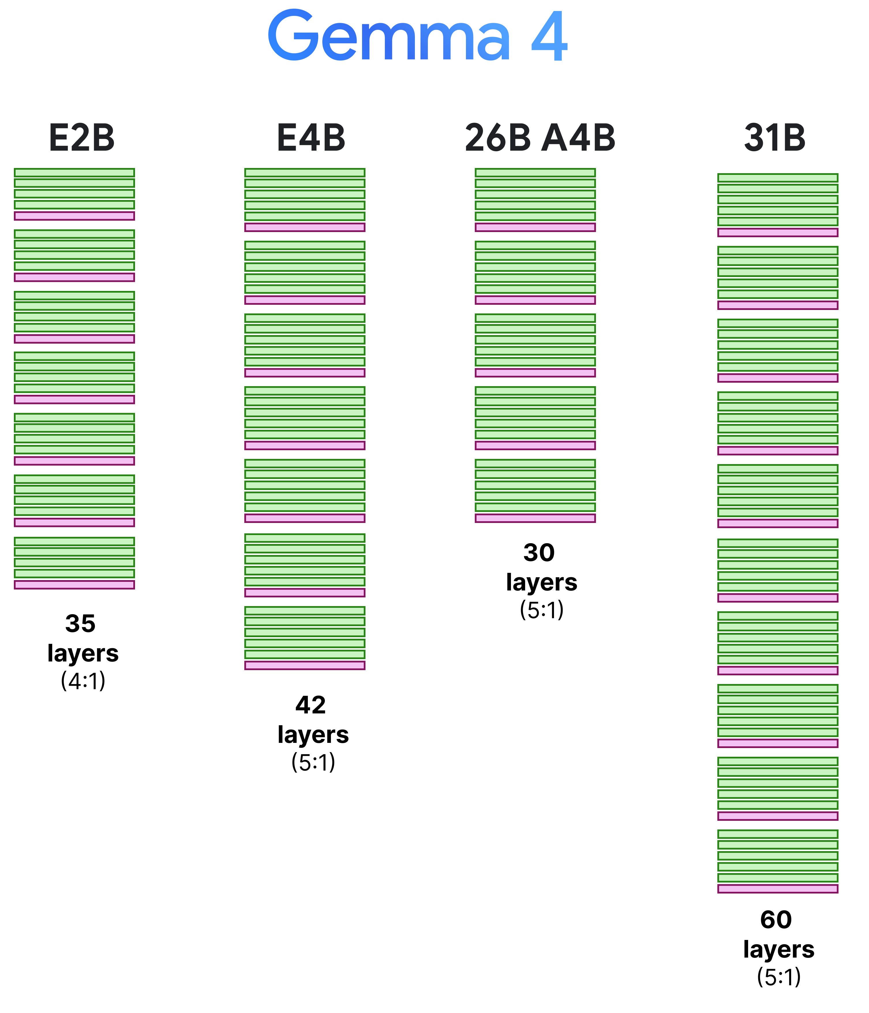
Note that the context window of the local attention layers were reduced from 1024 to 512 tokens to allow for further efficiency gains.

Making Global Attention more Efficient

Interleaving local attention with global attention is an interesting way of making a Large Language Model more efficient. However, it is not a free lunch. The global attention layers still attend to the entire context, which is a costly and slow process.

In this section, we explore various tricks that Gemma 4 uses to make those global attention layers more efficient!

Grouped Query Attention

Much like Gemma 3, these models use Grouped Query Attention (GQA) which allows the Query heads to share KV-values which reduces the amount of caching that needs to be done. The local attention layers use GQA and have 2 Query heads sharing one KV head.

With Gemma 4, the global attention layers are made more efficient by having 8 Query heads to share one KV head. This drastically reduces the caching needed of the KV values since global attention by itself already has a lot it needs to store (the entire context) compared to the small context of the local attention layers.

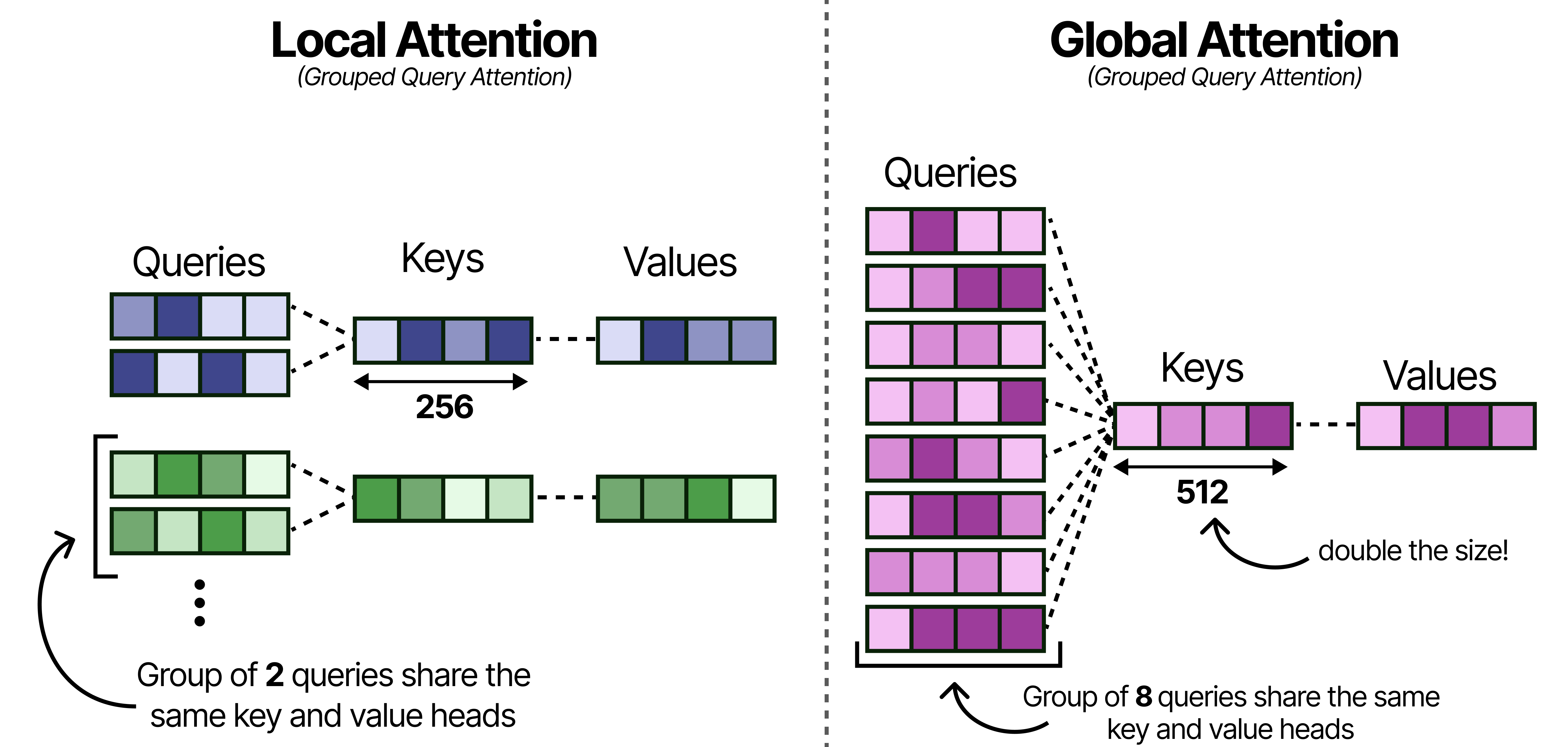
Note that reducing the number of keys and values per head may hurt performance and so to compensate for that, the size of the Keys was doubled!

Doubling the dimensions of the Keys does fill up the KV-cache quite a bit, so let’s explore another interesting trick for reducing the KV-cache.

K=V

Despite the improvements to the grouping in Grouped Query Attention, the global attention layers still take up quite a bit of memory since they attend to the entire sequence. Grouping into 8 queries helps a bit but there is more that can be done for efficiency!

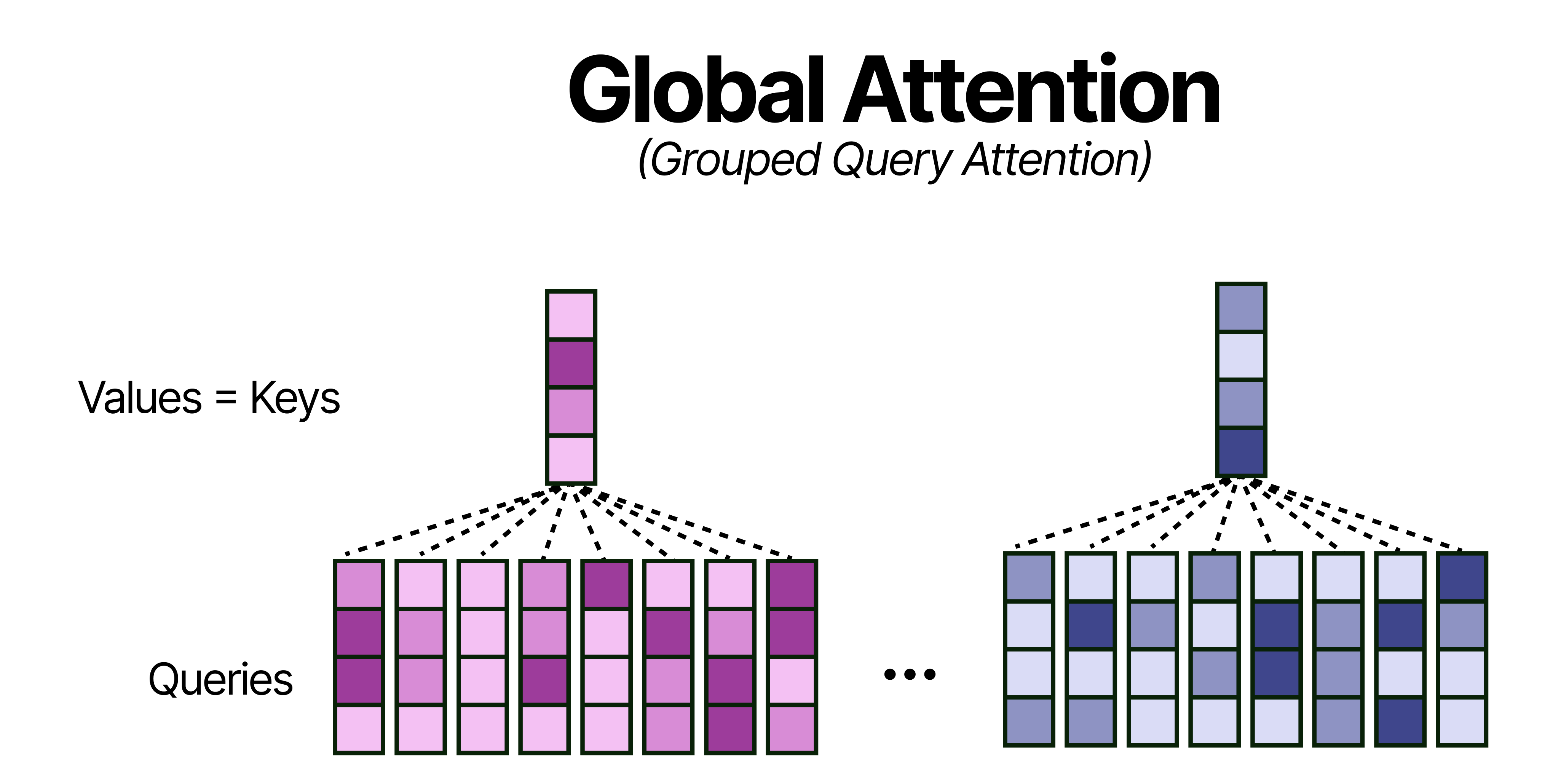
A neat trick, that does not hurt performance that much, is by using the Keys and Values only in the global attention layers. Effectively, this means that all Keys are equivalent to the Values which further reduces the memory requirements for the KV-Cache (or perhaps more accurately now the K-cache for the global attention layer).

p-RoPE

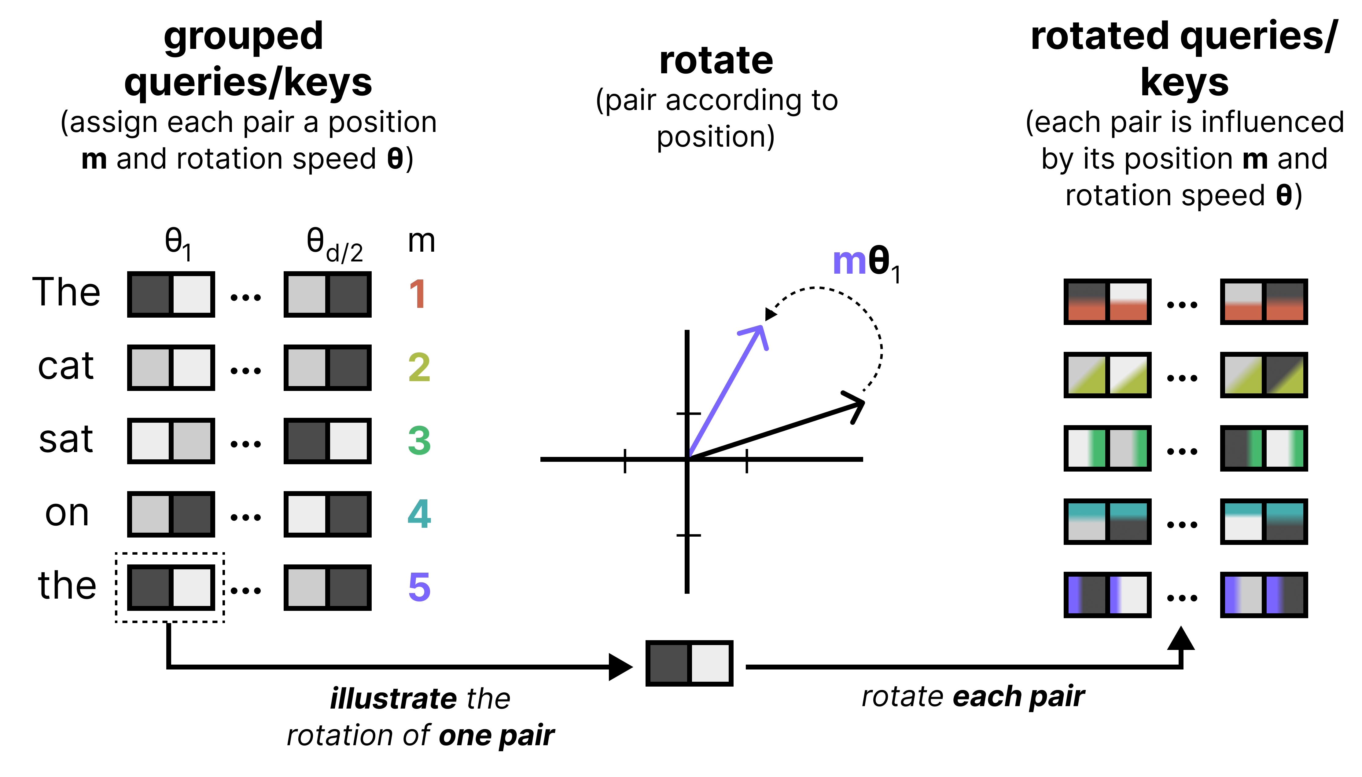
An important component of any Large Language Model is how it keeps track of the order of words in a sequence. One of the most common techniques is called Rotary Positional Encodings (RoPE). RoPE takes the Query and Key vectors and slices them up into pairs of two values. Each pair can now be seen as a vector in 2-dimensional space pointing towards a direction. RoPE rotates this direction slightly for each pair of values at decreasing speeds. The first pair has a large rotation compared to the last pair. This rotation allows the model to track the relative distances between words.

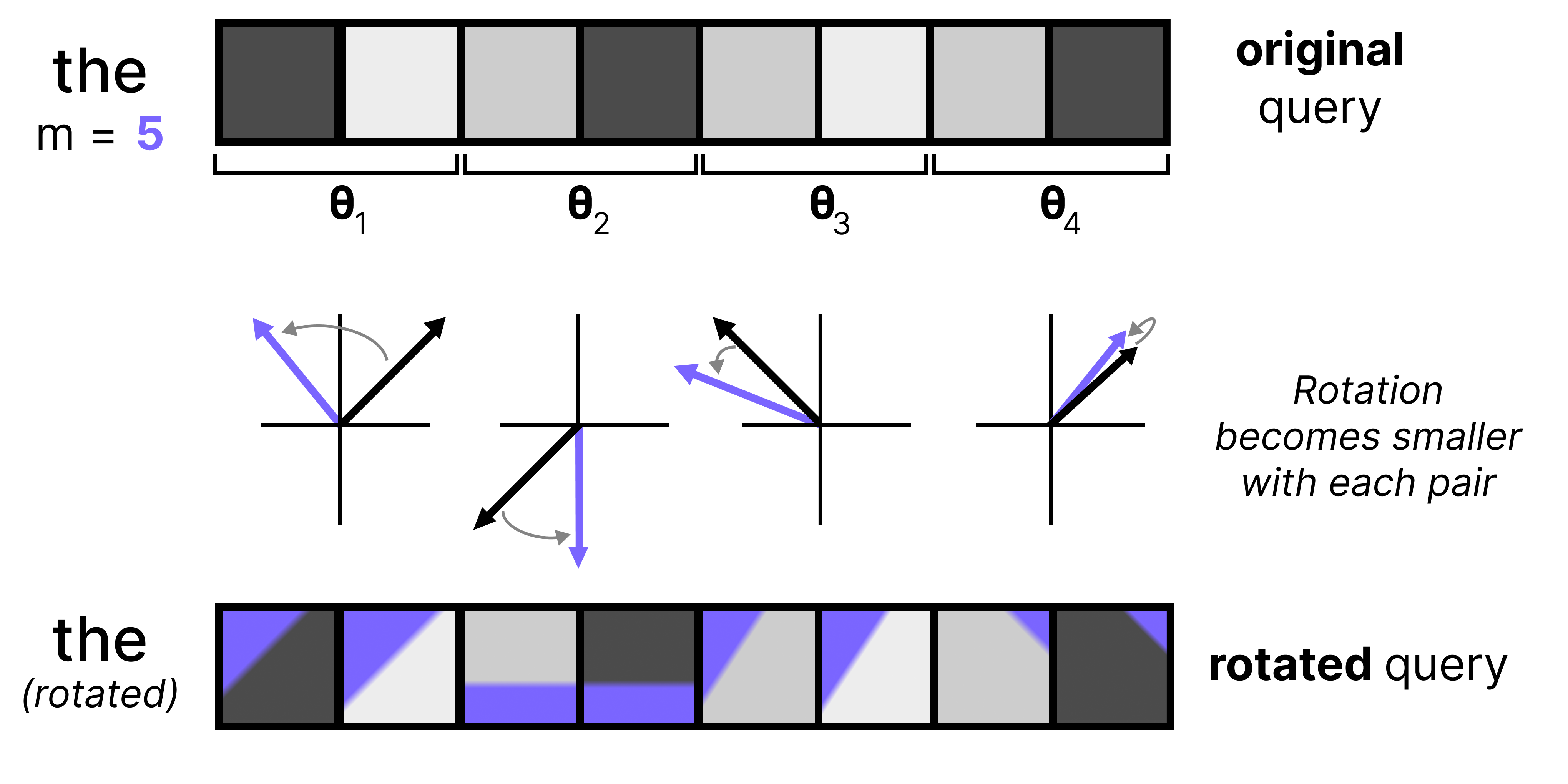
Let’s zoom in a bit on what happens if we were to rotate a query embedding. It first gets cut up into pairs of 2 and each subsequent pair is rotated. The rotation itself becomes smaller with each pair. This is referred to as the frequency, where a high frequency means that the rotation is quite large whereas a small frequency results in a smaller rotation.

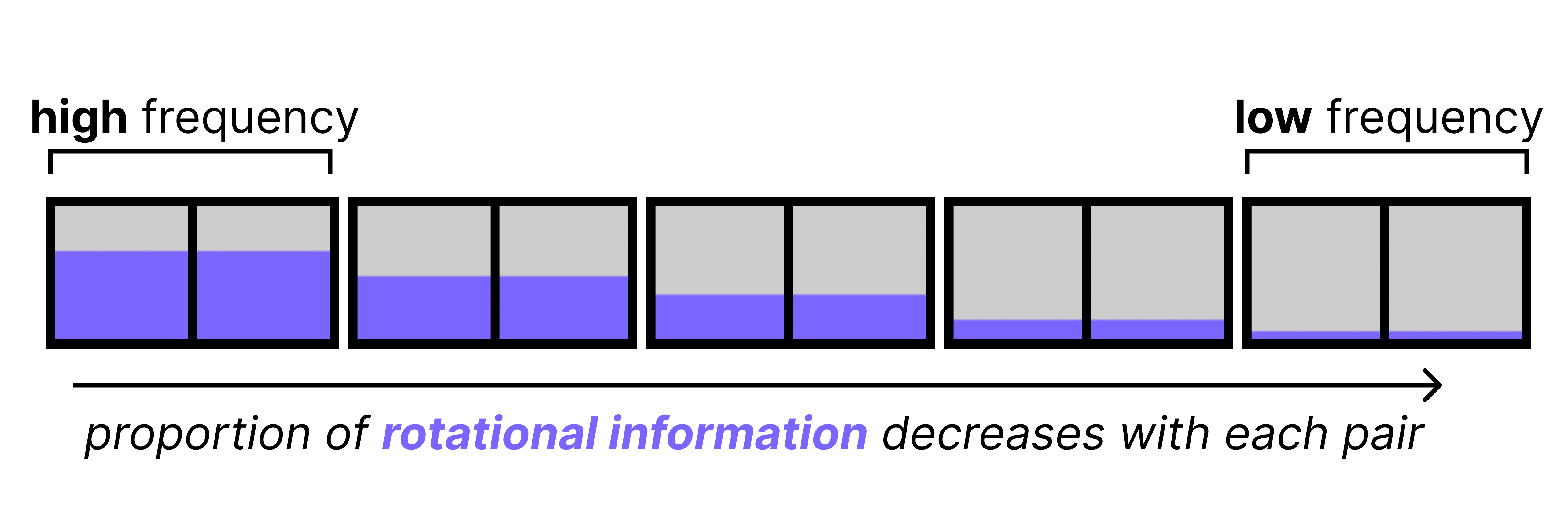
High frequency pairs are very sensitive to small changes in position due to the amount of information they were given at the first place (large rotation). They are great for tracking a word’s position. The low frequency pairs, however, are given a very slight rotation and barely move at all from word to word. Since these low frequency pairs only contain minimal positional information, and are closest to what the original KQ values were, they are more suitable for tracking semantic content. As such, they stay the most true to what they originally were (without positional information).

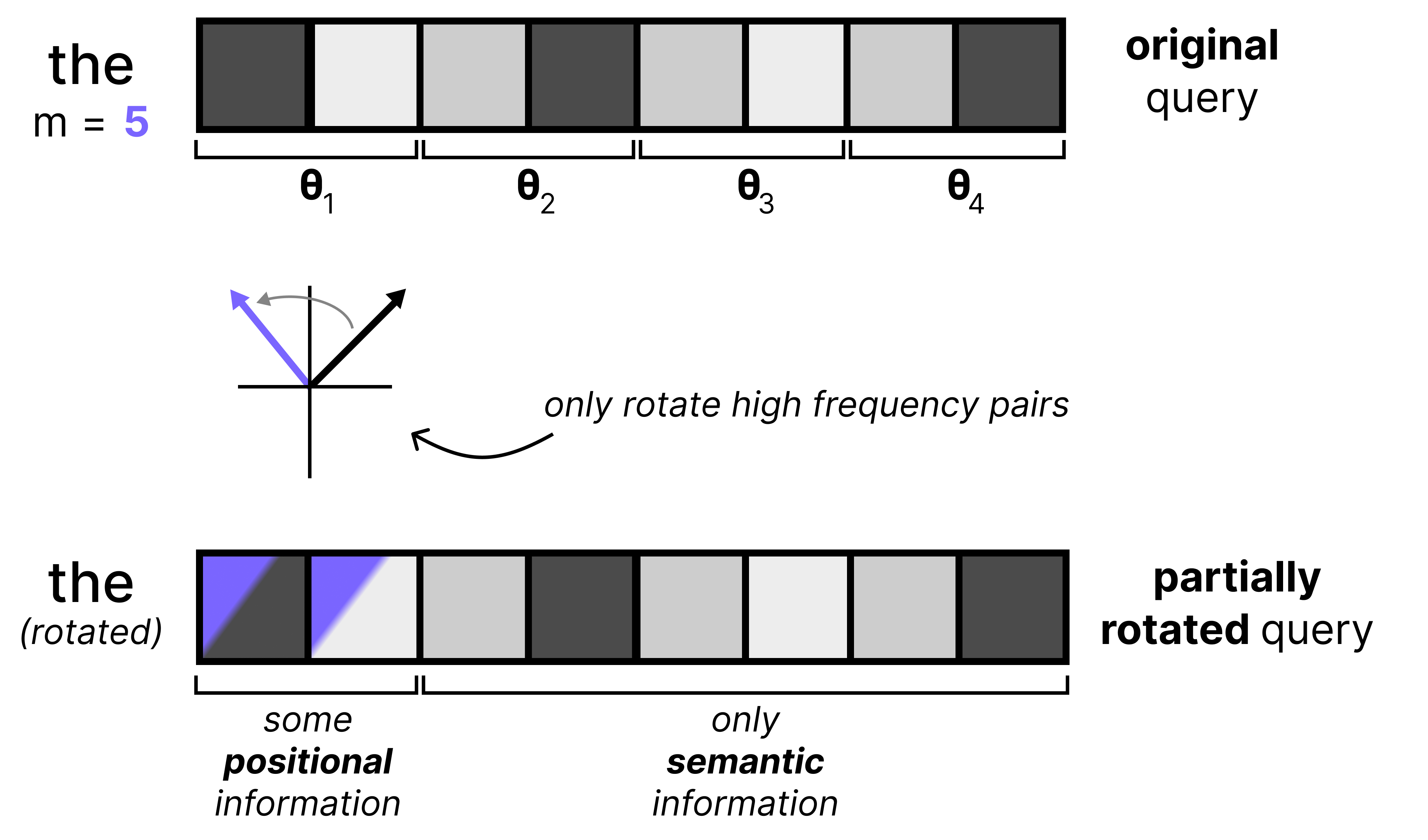
However, as it turns out, the high frequency pairs already contain sufficient positional information. The low frequency pairs contain just a little bit of positional information which is too little to be meaningful. It can even be harmful as models tend to use the low frequency pairs for semantic information, so the added positional information is just noise. Moreover, with long contexts the small rotations stack up and can eventually cause tokens that are far apart to become misaligned. This hinders the model’s ability to connect words across long sequences.

An elegant solution to this problem is by simply applying RoPE to only some of the dimensions of all vectors, which is called p-RoPE. If p is 0.25, then only the first 25% of pairs get positional information and all other pairs are set to 0. This allows the low frequency pairs to preserve meaning.

Gemma 4 uses p-RoPE on global attention layers since the context window is much higher there compared to the local attention layers. Moreover, p-RoPE is especially useful in global attention layers since large context windows may result in distances between tokens that the model hadn’t seen before. The space of all possible RoPE rotations is quite large with global attention versus local attention and by limiting the number of rotations, the model can do a much better job of handling a large context.

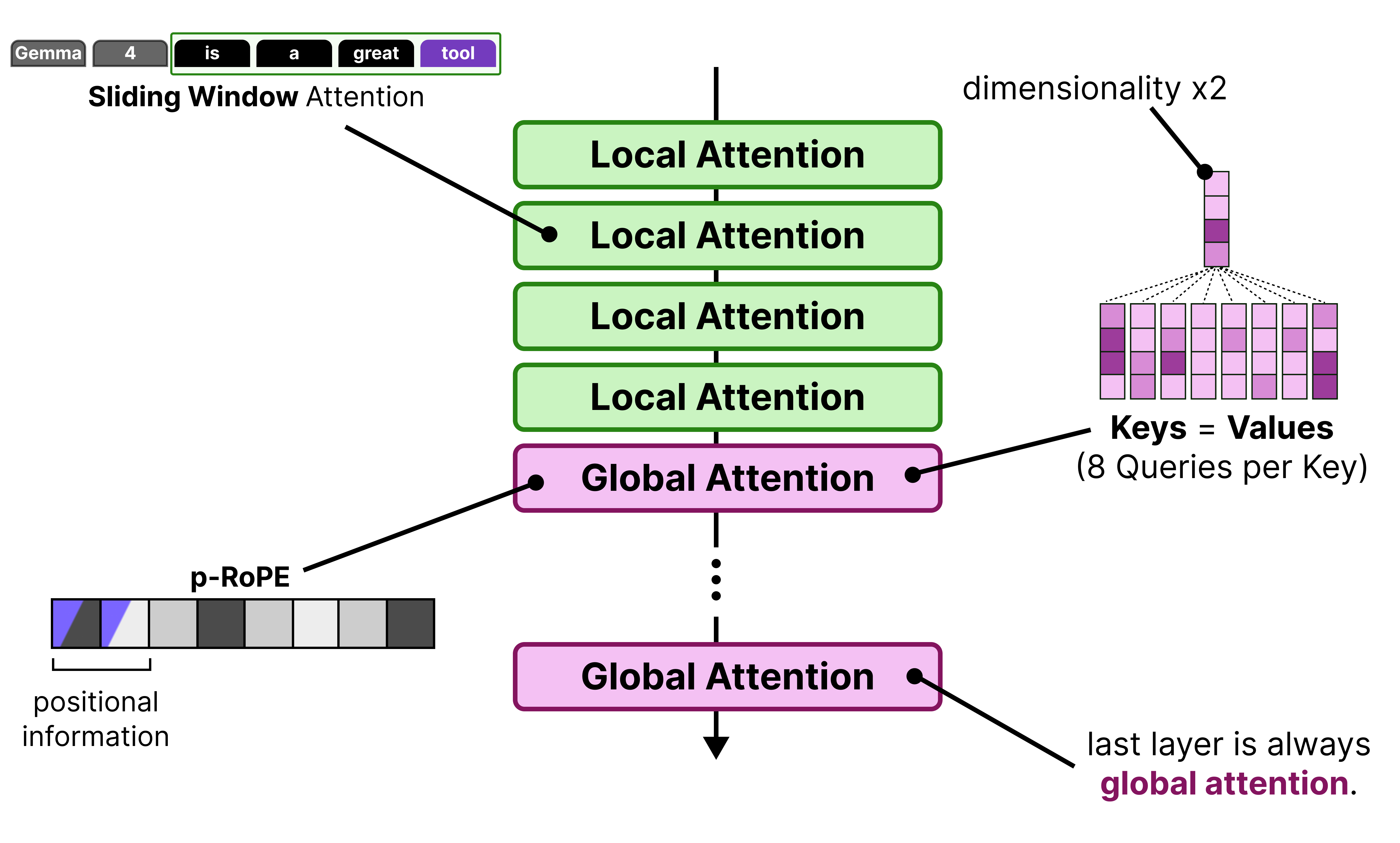
When we put everything together, you get the following improvements applied to the global attention layer:

• The final layer is always a global attention layer

• Has groups of 8 Queries per Key

• The dimensionality of the Keys are doubled

• Keys = Values

• p-RoPE where p=0.25

The Vision Encoder

A big component of the Gemma 4 releases are their multimodal capabilities. All variants support image inputs and allow for handling variable aspect ratios and resolutions!

What makes this possible is a Vision Encoder based on the Vision Transformer (ViT) to process the images. A ViT works similarly to a regular Large Language Model and instead of tokenizing text into sequences of words, it splits up the input image into sequences of patches. Each patch (a subset of the input image) is then passed a Transformer model which spits out an embedding per patch.

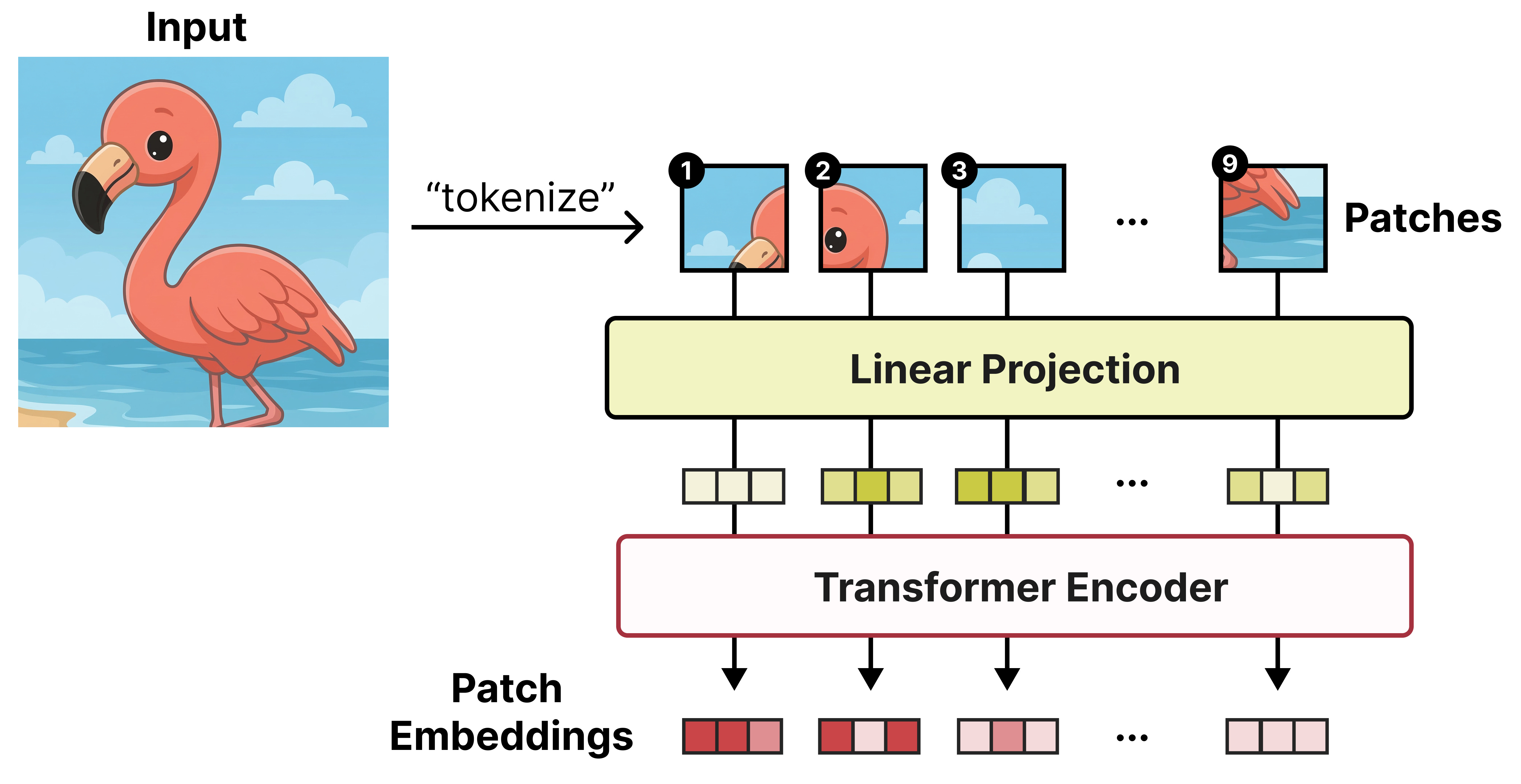
Each patch is a snippet of the original image and tends to be 16 by 16 pixels. The original paper was aptly named “An image is worth 16x16 words: Transformers for image recognition at scale”.

Variable Aspect Ratio

ViT assumes that the original image is a square that can be divided into patches of 16 by 16 pixels. However, there is a downside to this approach. When you process sequences of patches but the original image can be all different kinds of sizes, the position of a given patch (for instance patch 4) can mean different things depending on the proportion of the original image. For instance, if we assume that the original image will always be a grid of 3 by 3 patches, then patch 4 will always be in the middle. However, if the grid is dynamic and can be 2 by 4 patches for instance, then patch 4 will not be in the middle.

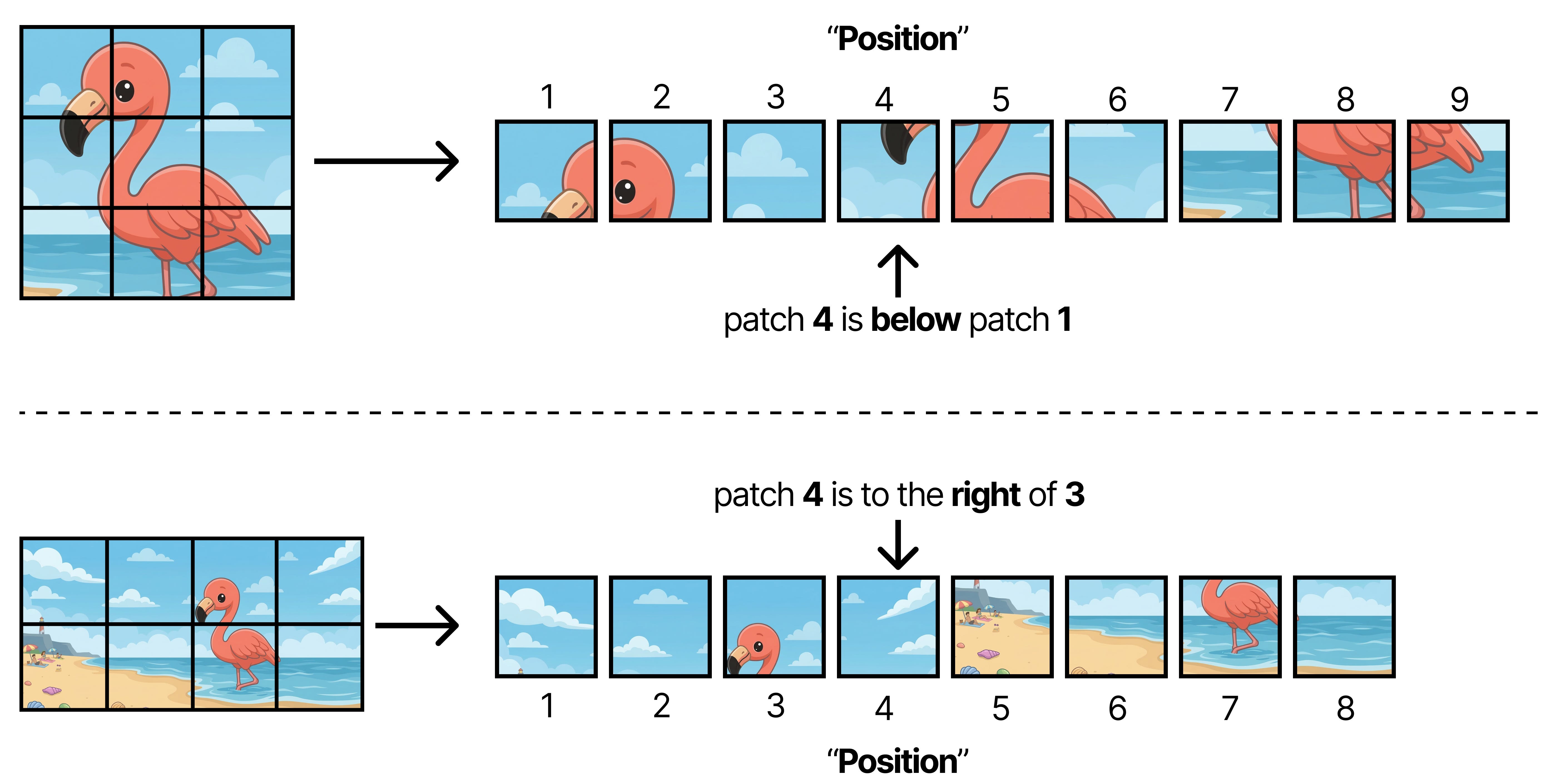
As such, applying RoPE is not straightforward anymore because the meaning of position (“Patch 4”) is now fully dependent on the aspect ratio of the original image.

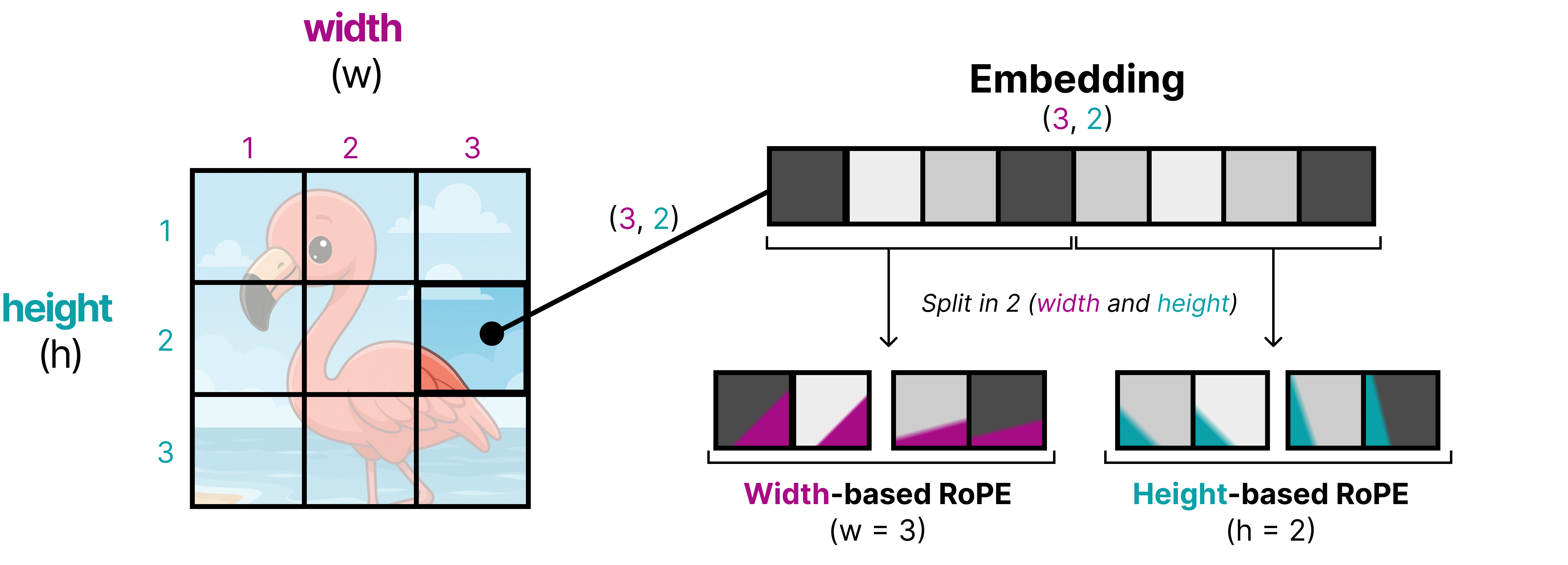
An interesting technique applied in Gemma 4 is to replace RoPE by 2D RoPE, which attempts to instill the 2D position of a patch into the positional embeddings rather than seeing them as a 1D sequence of patches. To do so, the embedding of a patch is first split up into two equal-sized parts. RoPE is applied to both parts of the embedding independently, but instead of using m as the position, they now use width (w) and height (h) to add positional information. That way, half of the embedding now contains positional information about its relative width position and the other half contains positional information about its relative height position.

Using 2D RoPE is not all that is needed to support variable aspect ratios. The original ViT, for instance, resizes the input to make them into squares so that the processed input nicely fits patches of 16 by 16 pixels. Imagine you have a wide image and you want to force it into a square… that would look either quite weird or crop away much of its content!

Gemma 4 introduces support for different aspect ratios by adaptively resizing the input image so that it still supports patches of 16 by 16 pixels. To maintain the original aspect ratio it will pad the image whenever there couldn’t be a perfect fit of a 16 by 16 pixel box.

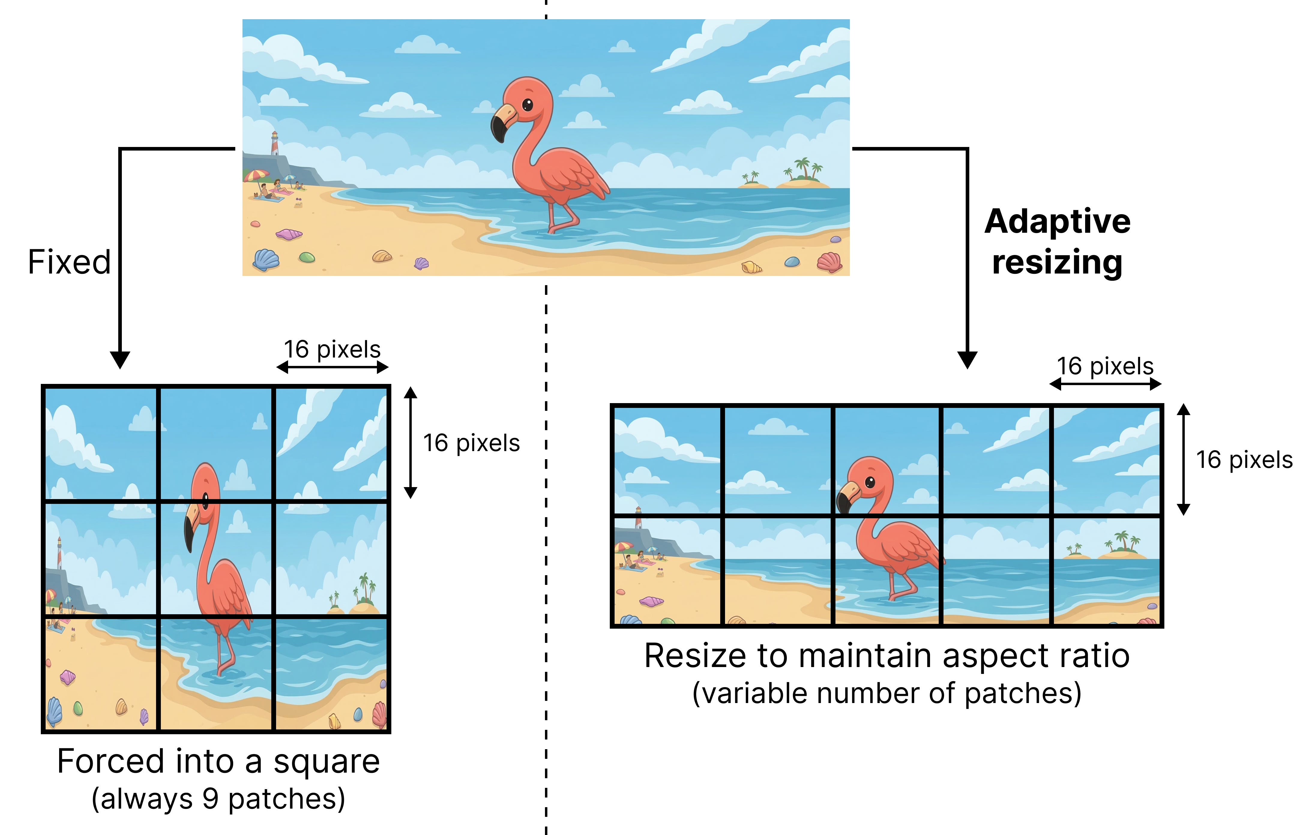
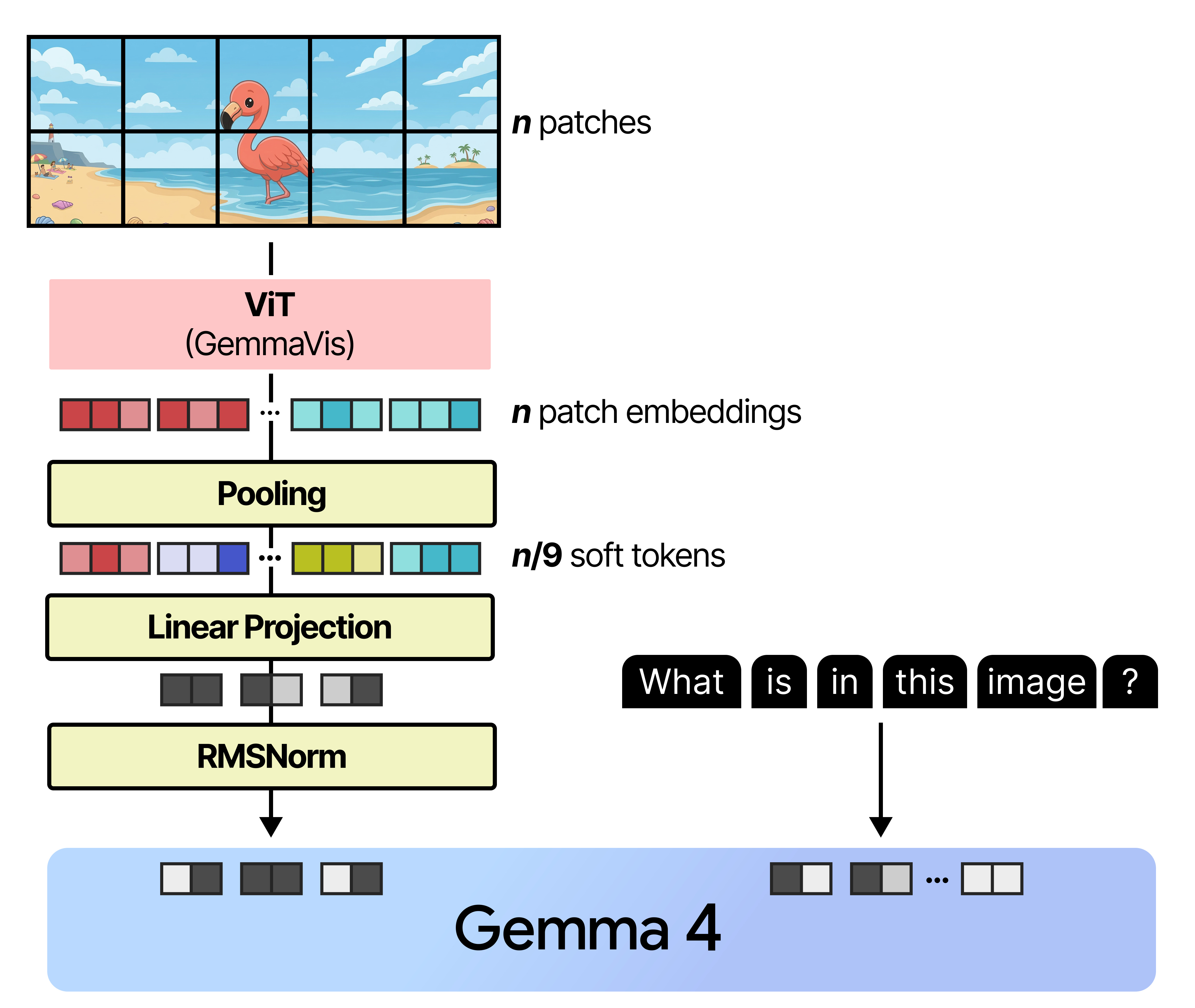
The original ViT typically assumed a fixed size for the square and therefore would always get back a fixed number of patches (9 in our example). The adaptive resizing method returns a variable number of patches, which can grow quickly in size. Therefore, the tokens generated by the ViT are pooled based on their spatial location. Patch embeddings close to each other get merged until a fixed number of patch embeddings are left.

Variable Resolution

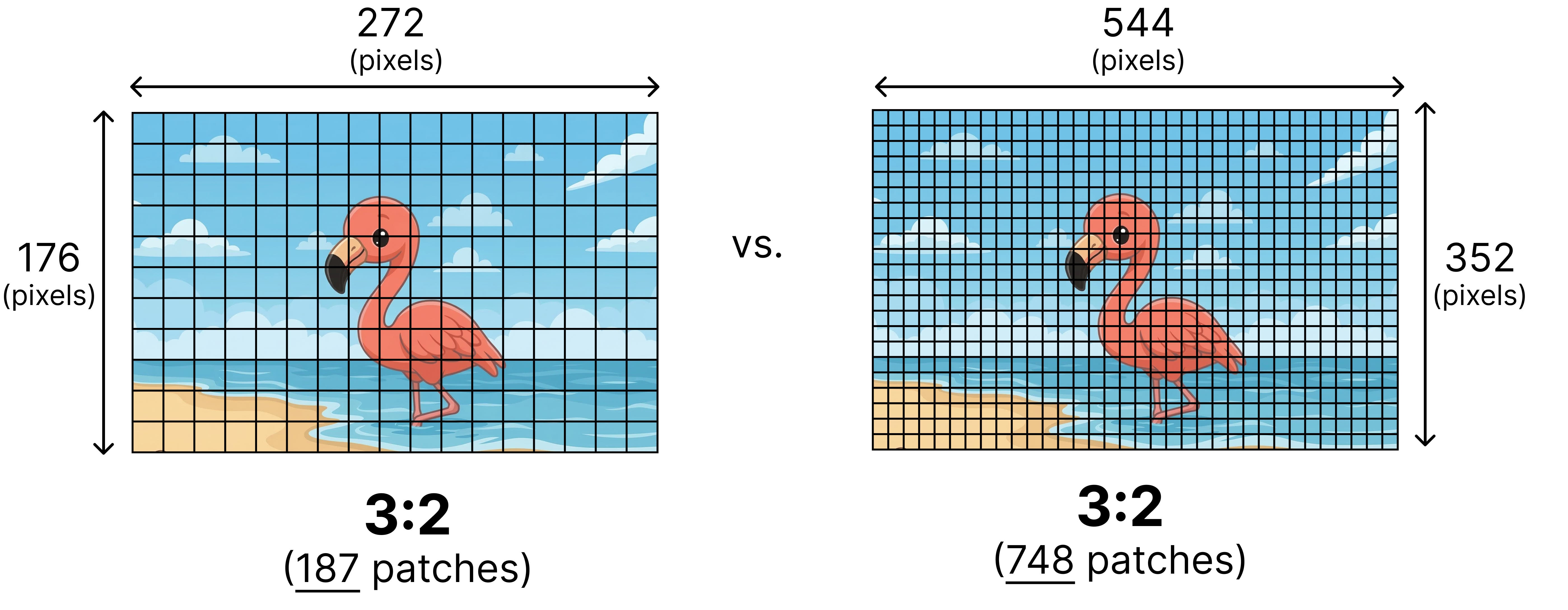
Although variable aspect ratios solve a bunch of problems, how do we decide the number of patches to use? Two images with the same aspect ratio can have different resolutions. Imagine you have two images with both an aspect ratio of 3:2 but one has a lower resolution of 272 by 176 and the other a higher resolution of 544 by 352.

One method would be to always decide on a certain fixed number of patches and resize the image accordingly. However, for certain tasks we might want to support higher resolutions, such as object detection and segmentation whilst for video you might be alright with smaller resolutions to speed up analyzing subsequent frames.

Gemma 4 supports different resolutions by introducing a soft token budget. This budget represents the maximum number of patch embeddings (also called soft tokens or visual tokens) are passed to the LLM to process. The user can decide between budget sizes of 70, 140, 280, 560, or 1120 tokens.

Depending on the budget, the input is resized. If you have a higher budget (like 1120 tokens), then your image can maintain a higher resolution and as a result will have many more patches to process. If you have a lower budget (like 70 tokens), then your image needs to be downscaled and you will have fewer patches that need to be processed. With a higher budget (and therefore more tokens), you can capture much more information than with a lower budget.

This budget determines how much the image is resized. Imagine you have a budget of 280 tokens, then the maximum number of patches will be 9 x 280 = 2,520. Why times 9? That’s because in the next step, every 3x3 block of neighboring patches are merged into a single embedding by averaging them.

The budget sizes roughly represent the following resolutions:

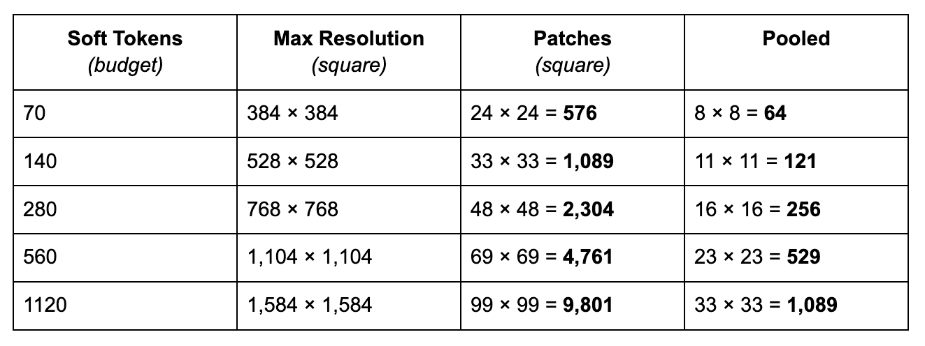
For simplicity, this assumes a square but with variable aspect ratio it can take different ratios and as a result, the patches will also have different dimensions. Also note how the soft tokens are smaller than the actual number of pooled embeddings, that is because the resolution should be multiples of 48 considering 3 patches of 16 pixels are pooled to a single embedding.

Below is an example of how an initially large number of patches gets averaged (also called pooling) into a lower number of patch embeddings (also called soft tokens).

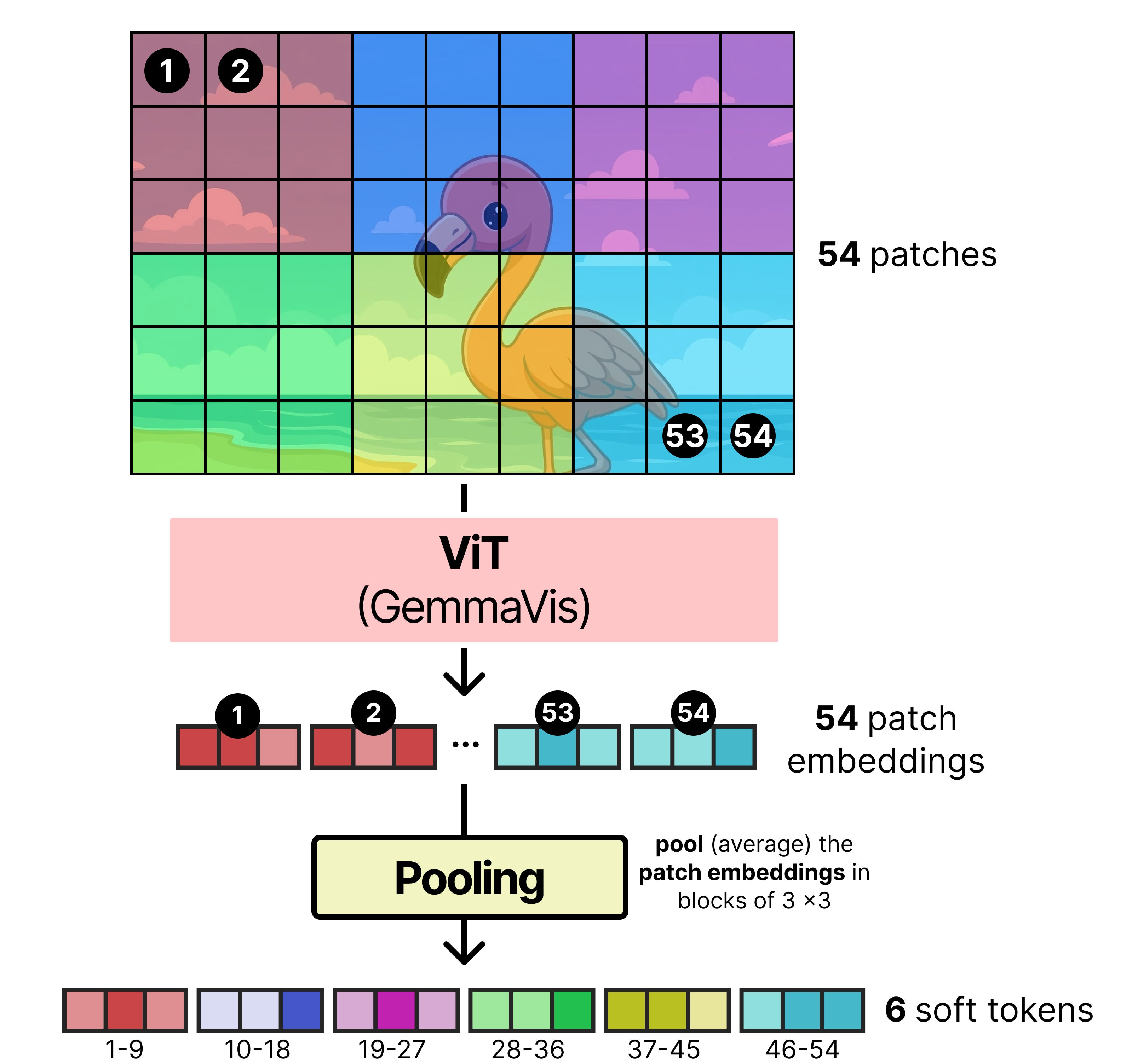
The pooled patches are typically smaller than the token budget because not every image will perfectly capture the maximum number of patches.

Linear Projection

The patch embeddings generated as a result of the image encoder cannot be given directly to Gemma 4. Like all language models, it expects the input embeddings to have a certain dimensionality to be able to process it. Ideally, you would also want its embeddings to occupy dimensional space in a similar way as the token embeddings such that they can be compared easily.

There is a nice example in the image below where you can see how a given image encoder creates an embedding that is much different from the token embedding created by the text encoder.

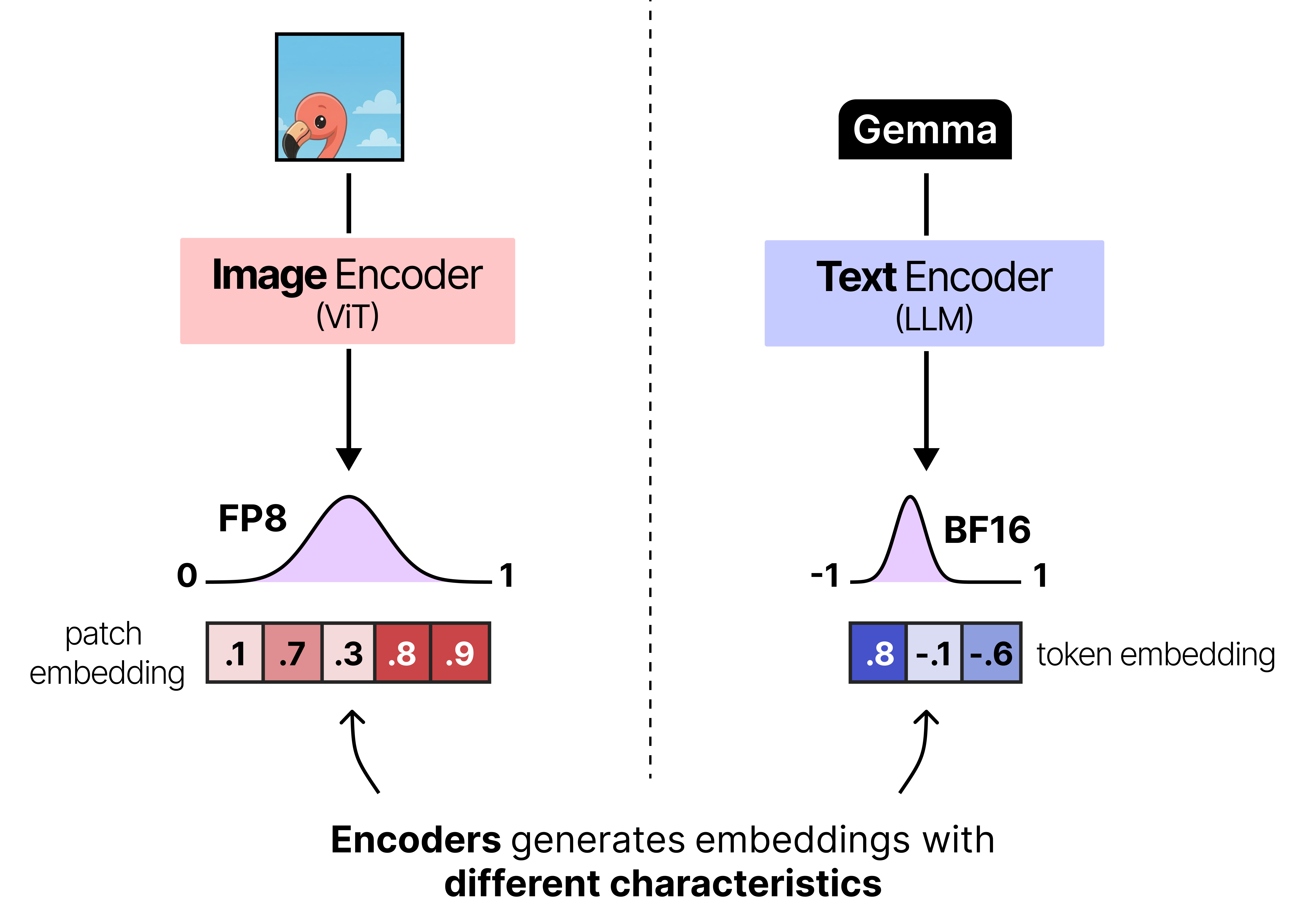
To make sure that the patch embeddings are aligned correctly with the token embedding the patch embeddings are typically projected using a small neural network so that they have the same dimensions and value distributions as what the language model expects. In Gemma 4, this projection is then followed by RMSNorm to match scale expectations of subsequent Transformer blocks.

And that’s how images are processed by Gemma 4! Note that to perform this linear projection, it is trained alongside Gemma 4 to make sure that the projected patch embeddings closely match what Gemma 4 expects.

Moreover, the smaller models (E2B and E4B) all use a vision encoder with 150 million parameters and all other models use a vision encoder with 550 million parameters.

Putting Everything Together

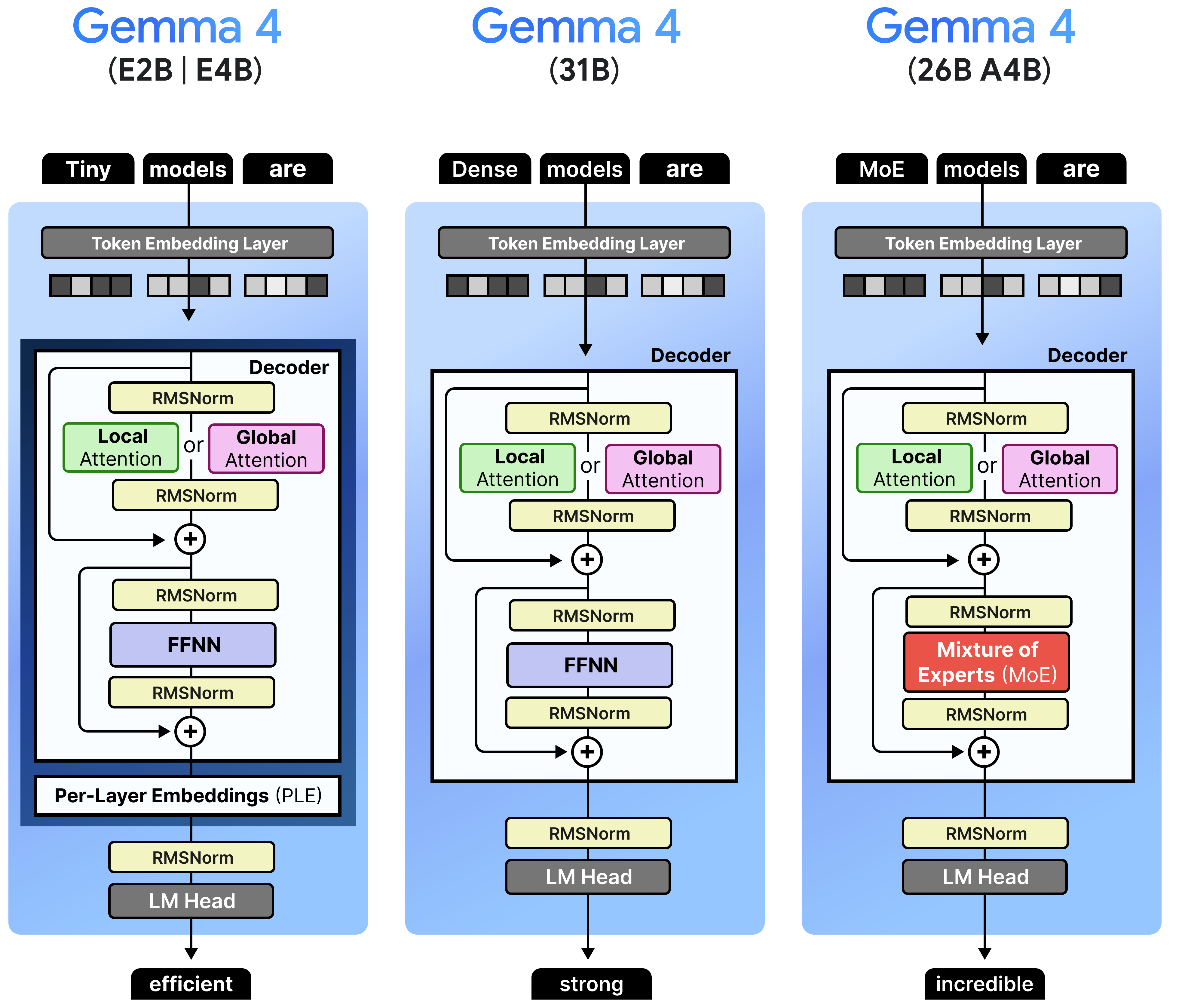
When we put everything together, the Gemma 4 architecture that all variants share, can be summarized into three major aspects:

• Interleaving Layers of Local and Global Attention

• Either Dense or Mixture of Experts

• Vision encoder

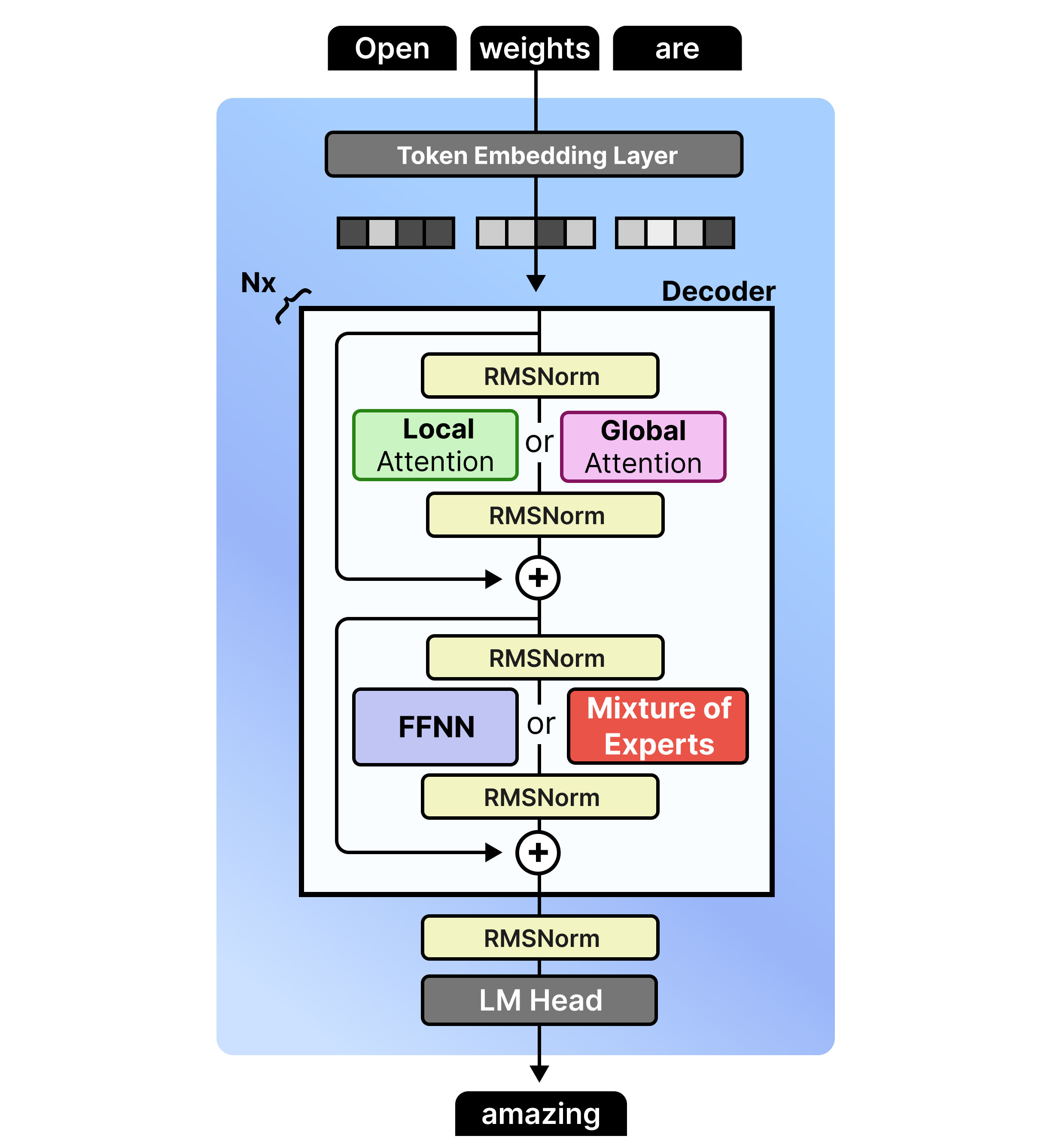
Note that the feedforward neural networks (FFNNs) are not interleaved with Mixture of Experts (MoE). Any Gemma 4 variants will have either one in all layers or the other.

Now that we have covered the main principles of each variant, let’s go into each set of models to explore them a bit more in-depth:

• Gemma 4 - 31B

• Gemma 4 - 26B A4B

• Gemma 4 - E2B and E4B

Gemma 4 - 31B - Dense

Despite the popularity of Mixture of Experts (which we cover later), the Gemma 4 family has a dense variant that is quite large with 31B parameters. This model is a nice representation of a more “vanilla” architecture amongst the Gemma 4 variants.

This model is architecturally quite similar to its Gemma 3 counterpart, namely the 27B variant. They both interleave local and global attention and have the same pre- and post- RMSNorm. What it does differently are the aspects we discussed before, like K=V and using P-RoPE. In particular, Gemma 4 - 31B has fewer layers (60 vs 62) but is a wider model.

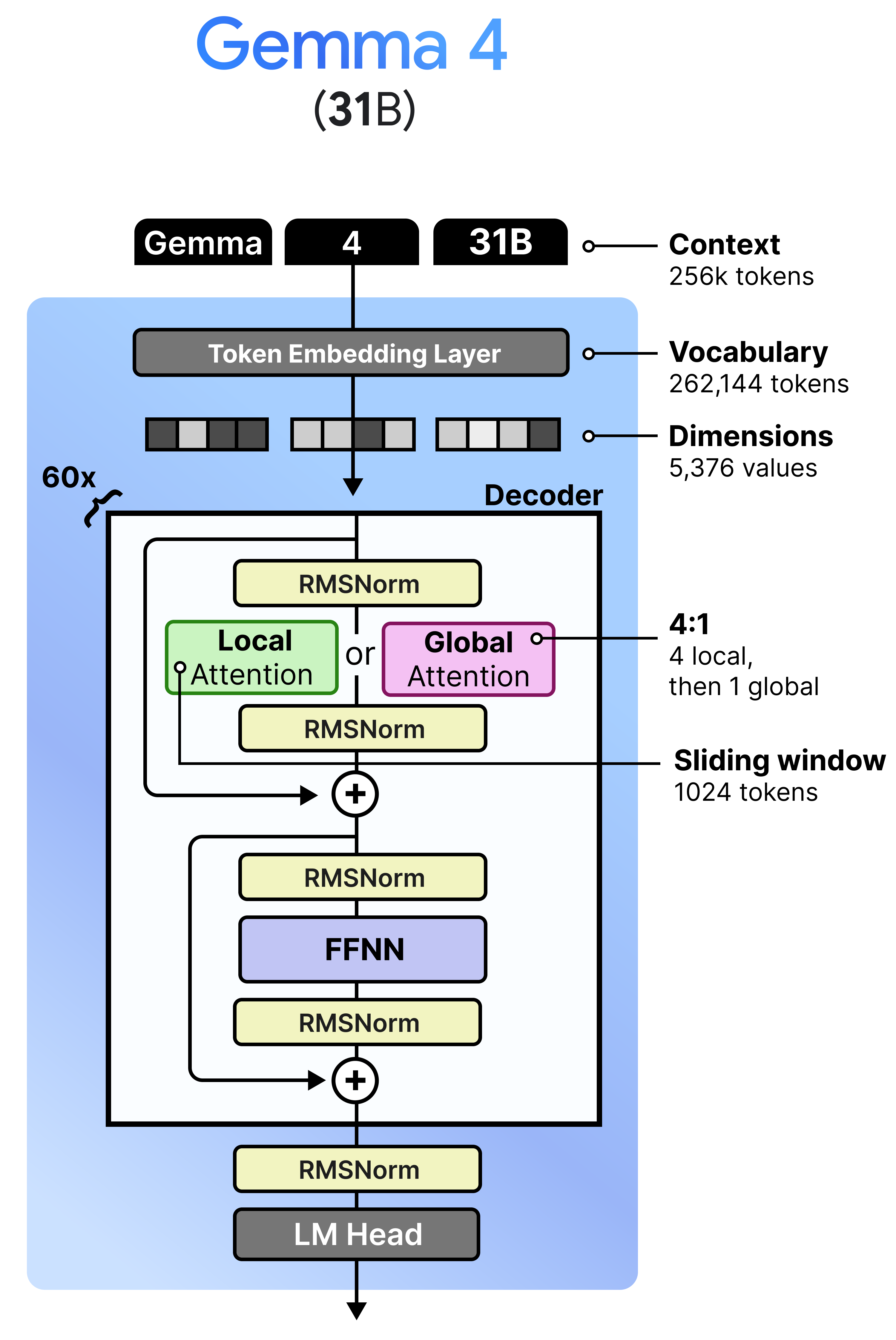
Unlike the Mixture of Experts model and the per-layer embeddings of the tiny models, this variant does not have a “magic” ingredient for us to explore. I think it is a nice representation of the “vanilla” Gemma 4 architecture and allows us to build on this to explore the other models.

Gemma 4 - 26B A4B - Mixture of Experts

Gemma 4 has a variant that contains “A” in its name, namely the 26 A4B model. The “A” stands for “active parameters” in contrast to the total number of parameters they contain. Specifically, the 26B A4B model contains in total 26 billion parameters (which are all loaded in memory) but only 4 billion parameters are used during inference. These are referred to as the “active parameters”. By only activating a subset of parameters, these models run much faster than their total number of parameters might suggest.

The architecture that makes this possible is called Mixture of Experts or MoE. Instead of using one big Feedforward Neural Network (FFNN), it uses several smaller ones and dynamically chooses which ones to process a given input.

As such, there are two main components to a MoE:

• Experts — A set of FFNNs that can process tokens but only a subset is activated at a time. They tend to be smaller than the FFNN in a dense (“regular”) model.

• Router — Determines which tokens are processed by which experts.

A given token embedding is processed in the MoE layer by first passing to the router which selects one or more experts to activate. To do so, expert probabilities are generated which allows for routing the token embedding. The selected experts update the token embedding as a Feedforward Neural Network normally would.

The probabilities allow for some experts to have a larger or smaller influence on the processed embeddings compared to other experts. As such, the processed embedding is multiplied by the expert probability.

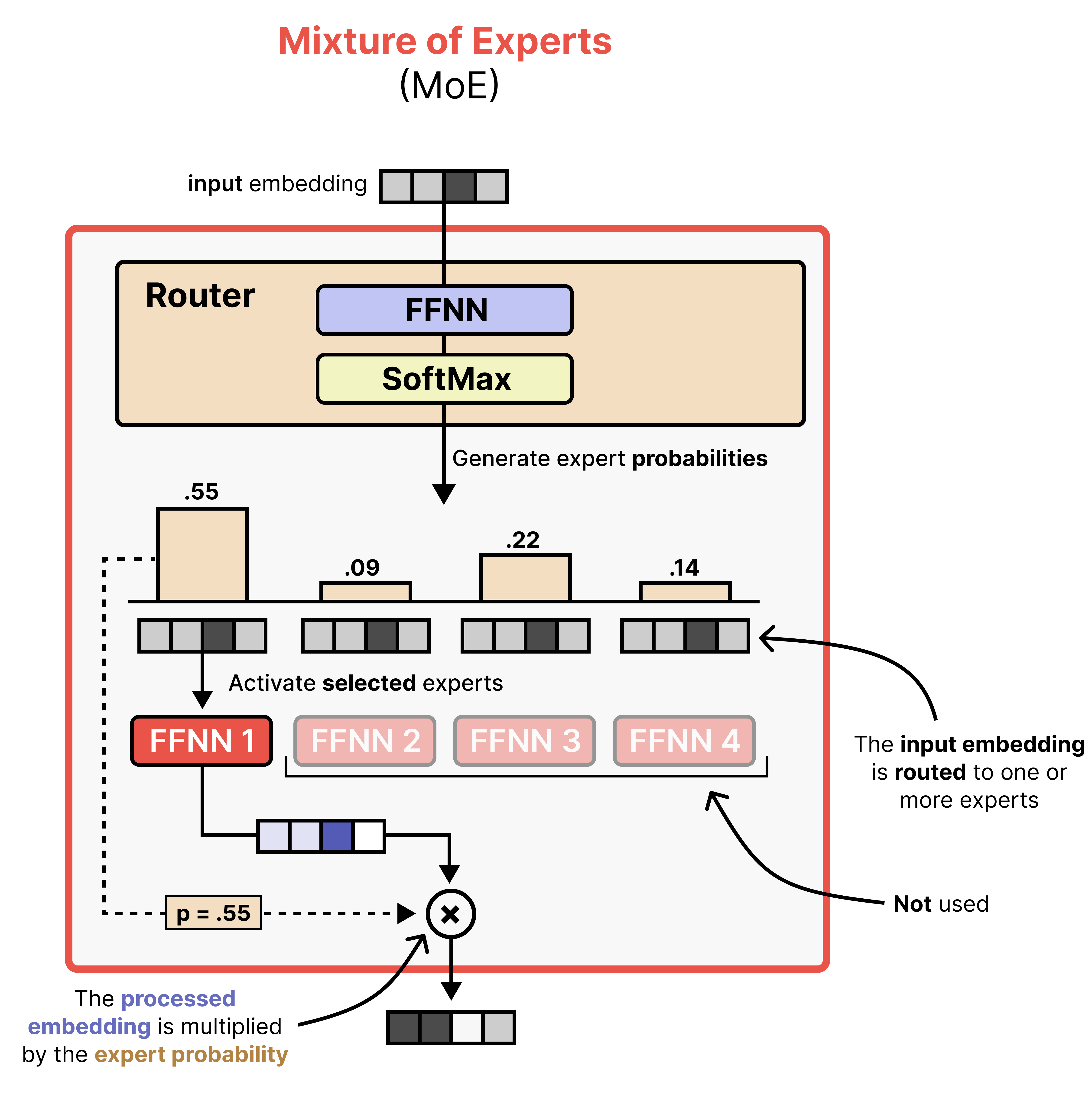
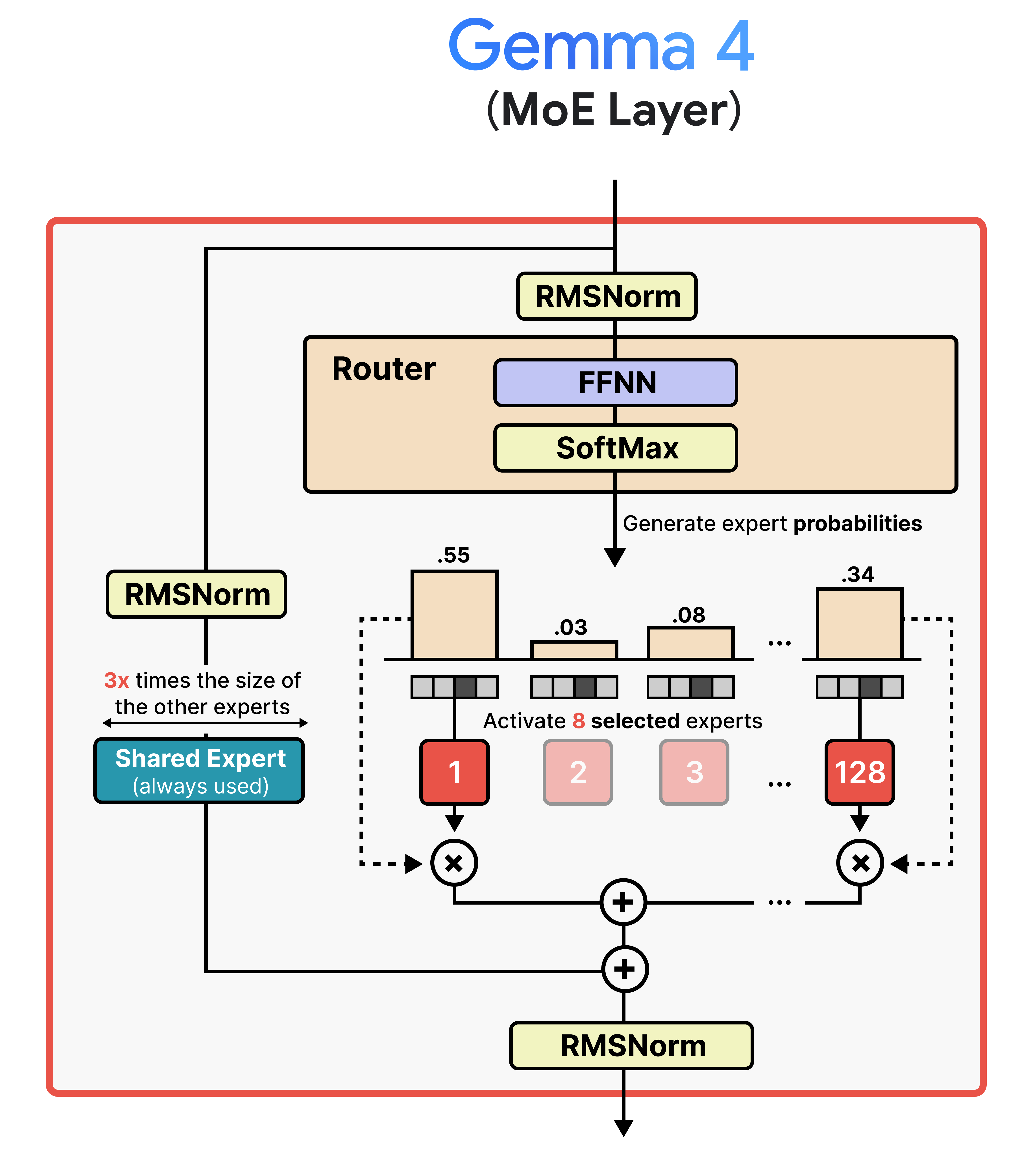
Although the visual shows a single expert, most MoE activate at least several and combine the result. In Gemma 4, the MoE variant has 128 experts that the router can choose from and 8 will be activated at a time.

Moreover, there is a shared expert. This expert will always be activated and used to process the input embedding. The underlying idea of having a shared expert is that it contains a lot of general knowledge that should always be activated, whereas the selected experts contain more fine-grained knowledge. In Gemma 4, this shared expert is three times the size to make sure it encompasses the necessary general knowledge.

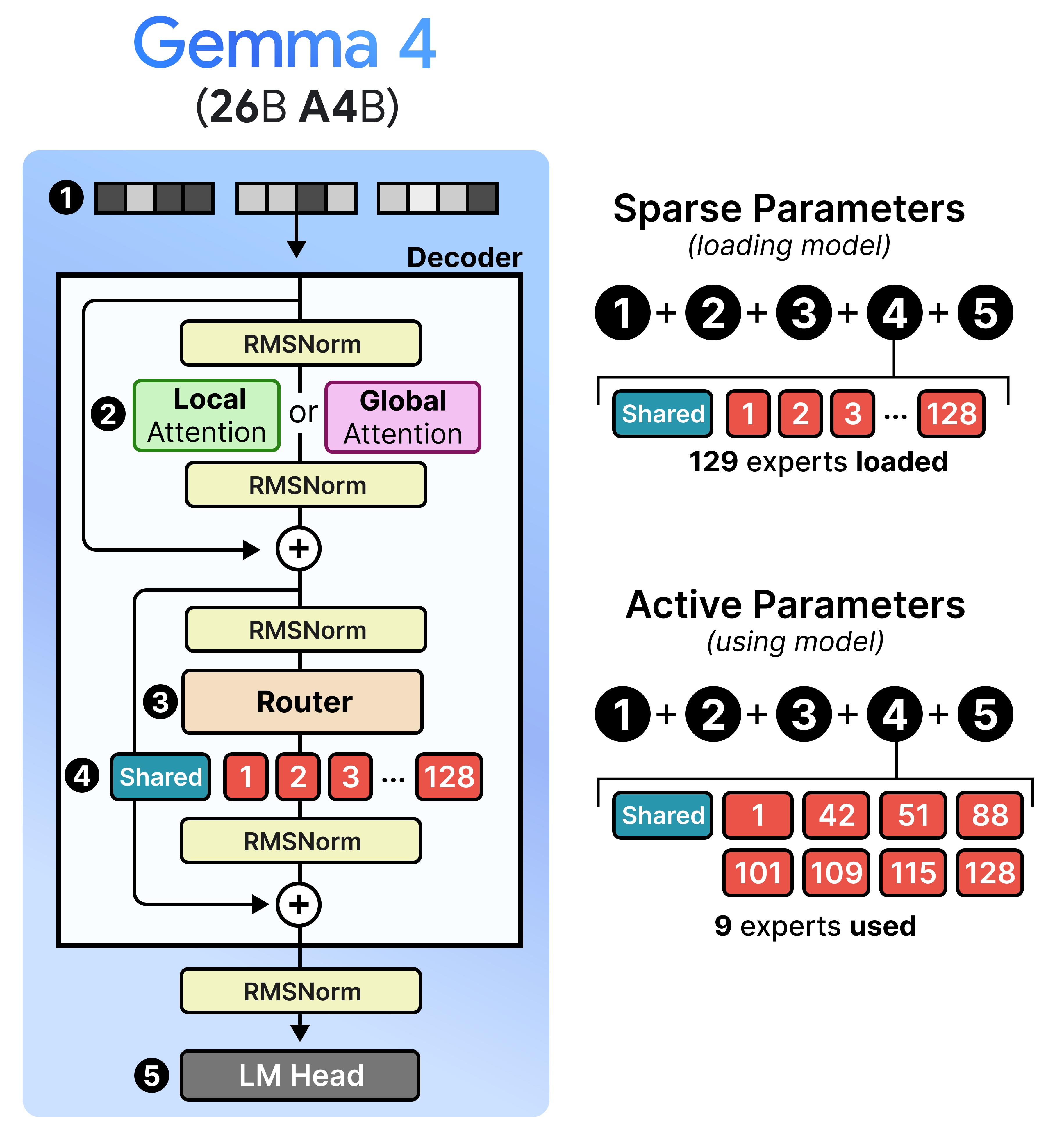
Now that you have a big picture of Mixture of Experts in Gemma 4, let’s explore a bit more in-depth what it means to have an efficient architecture with sparse and active parameters. The sparse parameters are every single parameter of the model which needs to be loaded into memory when you want to load the model. Gemma 4’s 26B billion parameter model for instance is quite large and you might think that it will run slow because of its big size. However, not all of its sparse parameters are actually used by your device (e.g., GPU) when you are running the model. With Mixture of Experts in Gemma 4, only 8 experts and 1 shared expert is actually used for intermediate calculations. All other 119 experts can take a backseat. These are the active parameters and represent the “A” in “26B A4B”. This means that although this model is large, it runs almost as fast as a 4B parameter model!

I’ve had a blast trying this model and I can tell you that it is a quite capable to run. However, you might want to use a smaller model if you want to run it on device like on your phone.

Gemma 4 - E2B & E4B - Dense

Gemma 4 has a variant that contains “E” in its name, namely the E2B and E4B model. The “E” stands for “effective parameters” in contrast to the total number of parameters they contain.

These models are very efficient and great for on-device use cases. What makes these models especially exciting is that they contain an additional audio encoder for processing audio alongside text and images.

Before we go into the specifics of the audio encoder, let’s first explore this “E”!

Per-Layer Embeddings

An interesting component of the smaller Gemma 4 models is the “E” in “E2B” and “E4B”. It stands for “effective” and is in a way similar to sparse versus active parameters that we explored in Mixture of Experts. “Effective” essentially means that these parameters are used for computation and loaded on to your (V)RAM whereas the other parameters (a lookup table with embeddings) is used only once to quickly find related embeddings.

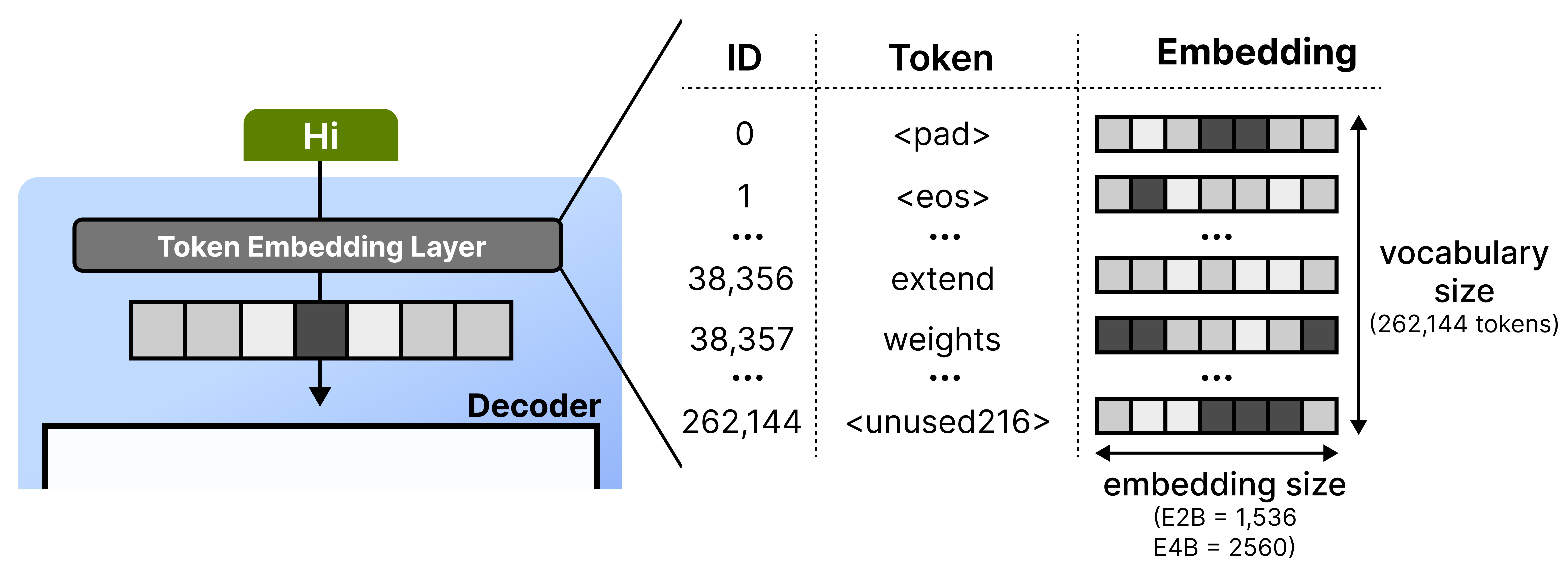
To explore what this means in practice, let’s first cover what happens at the token embedding layer. Whenever it receives a given token, it looks up its embedding using a lookup table. This table can be quite large since it has to store an embedding for each word in its entire vocabulary. Gemma 4 E2B, for instance, has 262,144 tokens each with an embedding size of 1536 dimensions.

Then, the embeddings for each token gets put through stacks of decoder blocks and iteratively processed. To improve the capabilities of a model, you would normally just add a couple of layers or more parameters. Bigger models tend to outperform smaller ones.

Instead of adding parameters to the model itself, a clever trick is to create an additional set of embeddings at every single layer. It is a bit simplified but imagine that embedding for the token “cat” might emphasize at:

• Layer 2 - “I am a noun, usually followed by a verb.”

• Layer 18 - “I am a small animal and related to terms like ‘pet’ or ‘feline’.”

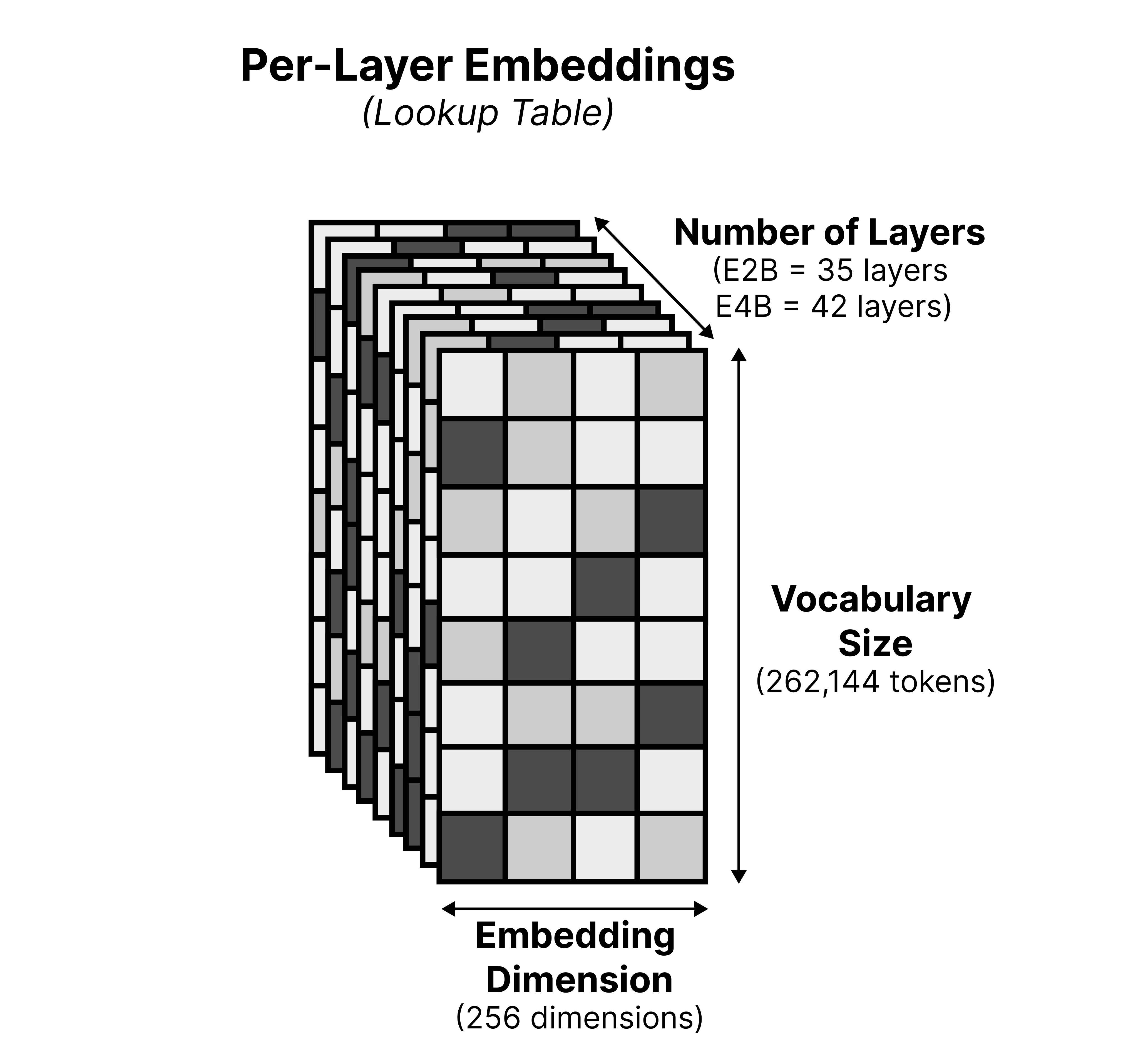
These embeddings are quite a bit smaller (256 versus 1536 dimensions in E2B and 2056 in E4B) than the original lookup table to save storage. As a result, we now have a lookup table of 262,144 tokens x 256 dimensions x N layers. The benefit of having a larger lookup table is that we can store important information on flash storage rather than needing valuable (V)RAM which is meant for computations in the model.

These are called Per-Layer Embeddings (PLE) and as the name suggests, are embeddings that used for specific layers.

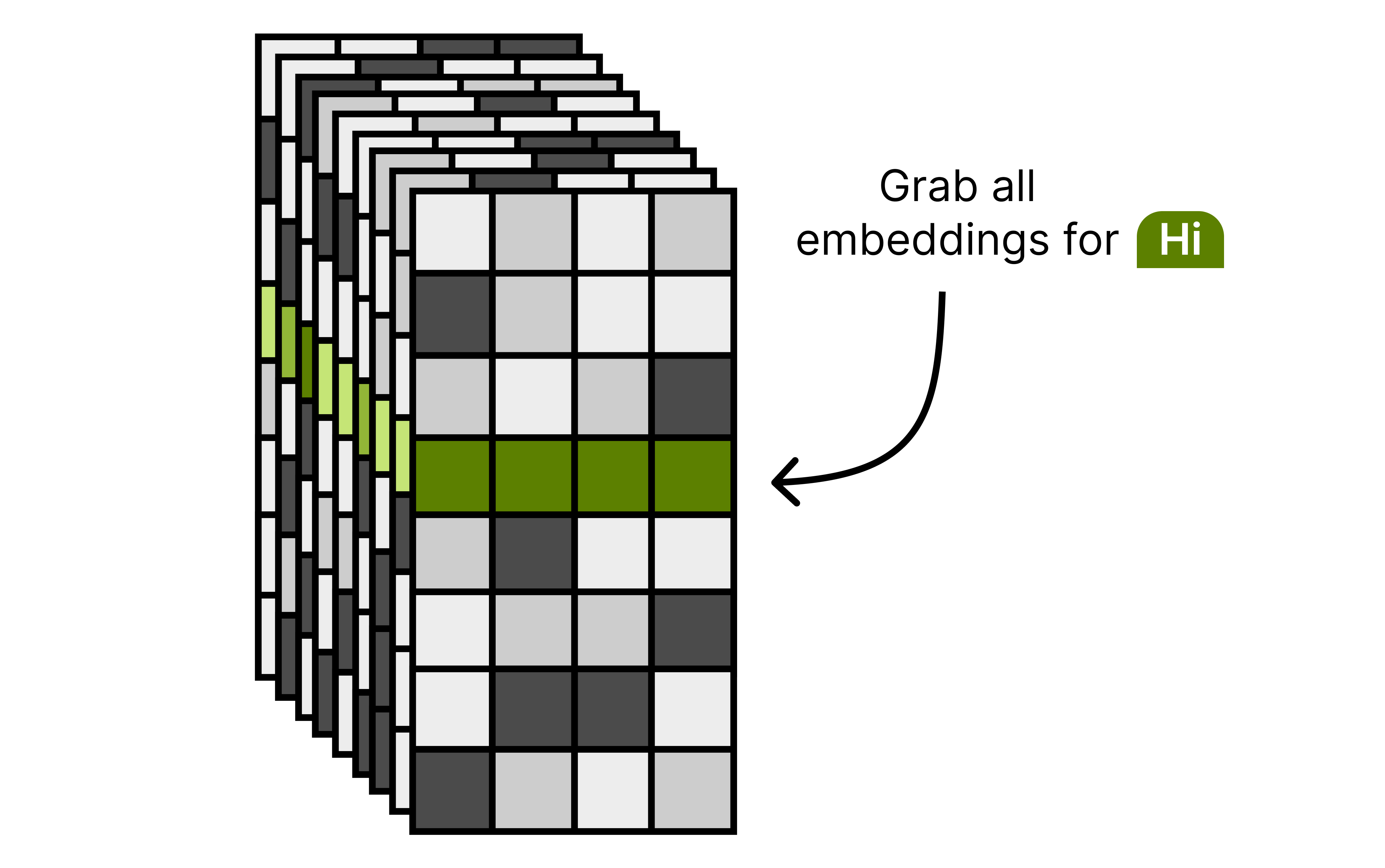
At the start of inference, the model grabs the set of embeddings for each input token. Each input token will have an embedding per layer to be used at that specific layer. Note that this lookup is done only once during inference, making this action quite compute efficient since there is no need to lookup the embeddings every time a layer is activated.

These embeddings are processed between each set of decoder blocks. Here, are gating function is used to decide how to weigh each value in a chosen embedding. This allows the model to additionally focus on certain parts of the embedding retrieved from the lookup table. The resulting embedding, still of dimensionality 256, is then projected up to match the original embedding size (1,536 for E2B and 2,560 for E4B).

After a normalization layer, this weighted representation is then combined with the original output of the previous decoder block. This allows for the processed signal to be “reminded” of what the token embedding represents, rather than it being mixed through a bunch of layers and getting a lot of context added to it.

The model can now focus its internal dimensions on making sense of the tokens rather than needing to carry around information from the bottom layer. This makes the existing layers much more efficient and expressive than they would be on their own.

But more importantly, these per-layer embeddings, albeit being quite large (262,144 x 35 x 256) are stored in flash memory. Storing it in (V)RAM would be a waste considering we only need a couple of embeddings during inference. Therefore, the “E” in “E2B” and “E4B” relate to all parameters except for the per-layer embeddings.

This is an elegant technique that allows these models to run on smaller devices, such as cellphones. There, the RAM is extremely valuable and limited, so anything you can do to minimize its usage is a welcome addition.

Audio Encoder

The smaller models (E2B and E4B) can also handle audio inputs and are nicely suited for tasks like automatic speech recognition and translation. Much like the vision encoder, the audio encoder transforms the raw audio input into embeddings that can be processed by Gemma 4.

There are several steps to this process but let’s start at the beginning. A common process in converting raw audio into tokens and their embeddings is through a three step process:

1. Extract features – Features are extracted from the raw audio through a mel-spectogram which is a 2D visual representation of the raw audio. It represents time (horizontal axis) and frequency bands (vertical axis).

2. Group into chunks – The mel features are grouped into chunks as a starting point for the sequence of tokens.

3. Downsample chunks - The chunks are overlapped and processed by two 2-dimensional convolutional layers to shorten the sequence length. As such, it converts the 2D chunks into a sequence of embeddings (also called “soft” tokens to represent the continuous nature of the token).

Fun fact: I recorded audio myself and created the mel spectogram for this visual!

This process is much like the linear projection of the image patches to create embeddings. They still need to be processed subsequently by an encoder so that the embeddings are filled with contextual information. The audio encoder used in Gemma 4 is called a conformer and is much like a regular Transformer Encoder but also uses a convolutional module to process the soft tokens. A nice comparison is between the dense Gemma 4 31B and how the Conformer is implemented. Note how it produces embeddings rather than tokens.

Much like the vision encoder, the embeddings produced by the Conformer are projected onto the dimensional space of the embeddings that Gemma 4 would expect. Otherwise, you get a mismatch in embedding size which cannot be processed by Gemma 4.

This gives us a pipeline that feels quite similar to what we explored with the vision encoder!

Multi-Token Prediction (MTP) with Gemma 4

To improve the inference speed of the Gemma 4 models, a new series of autoregressive “drafter” models has been released alongside the main lineup (E2B, E4B, 31B, and 26B A4B). Instead of solely relying on the primary Gemma 4 models (referred to as the “target” models), the draft model predicts several tokens in the time it takes the target model to process just one. This technique is also known as speculative decoding.

After the drafter has predicted multiple draft tokens, the target model now only has to verify those suggested draft tokens. The verification is done in parallel thereby drastically speeding up inference. It reduces the number of forward passes the target model has to do for each token. Because our drafter generates a sequence of tokens for verification, we refer to it as the Multi-Token Prediction (MTP) head.

The draft models released for the Gemma 4 family are small and introduce several enhancements to improve the quality of drafted tokens and to further speed up inference, like using the target model activations and KV-cache to get better predictions.

These enhancements result in significant decoding speedups while guaranteeing similar quality, making these checkpoints perfect for low-latency and on-device applications.

There is a lot to unpack here, so let’s go through speculative decoding, MTP, and the drafters!

What is Speculative Decoding?

Gemma 4 models generate text autoregressively and produce one token at a time. Roughly the same amount of compute is needed for each token, regardless of how difficult it is to predict a given token. As such, this can be an unnecessarily slow process when the tokens are quite easy to predict.

Imagine that the larger model is generating text and has already created “Actions speak”. For those that recognize the start of this sentence, it is a common proverb in the English language and extends to “Actions speak louder than words.”. Since it is quite common, smaller models are likely to generate the exact same completion (“louder than words”) as a larger model would. As such, it would be a waste of time and compute for the larger model to predict “louder than words” one token at a time.

With speculative decoding, we can use a smaller draft model to predict several tokens ahead of time. The draft model will receive the same input “Actions speak” and still autoregressively predict a number of tokens, let’s say four tokens. The drafted tokens are generated much faster than the larger model would as the draft model is only a fraction of its size.

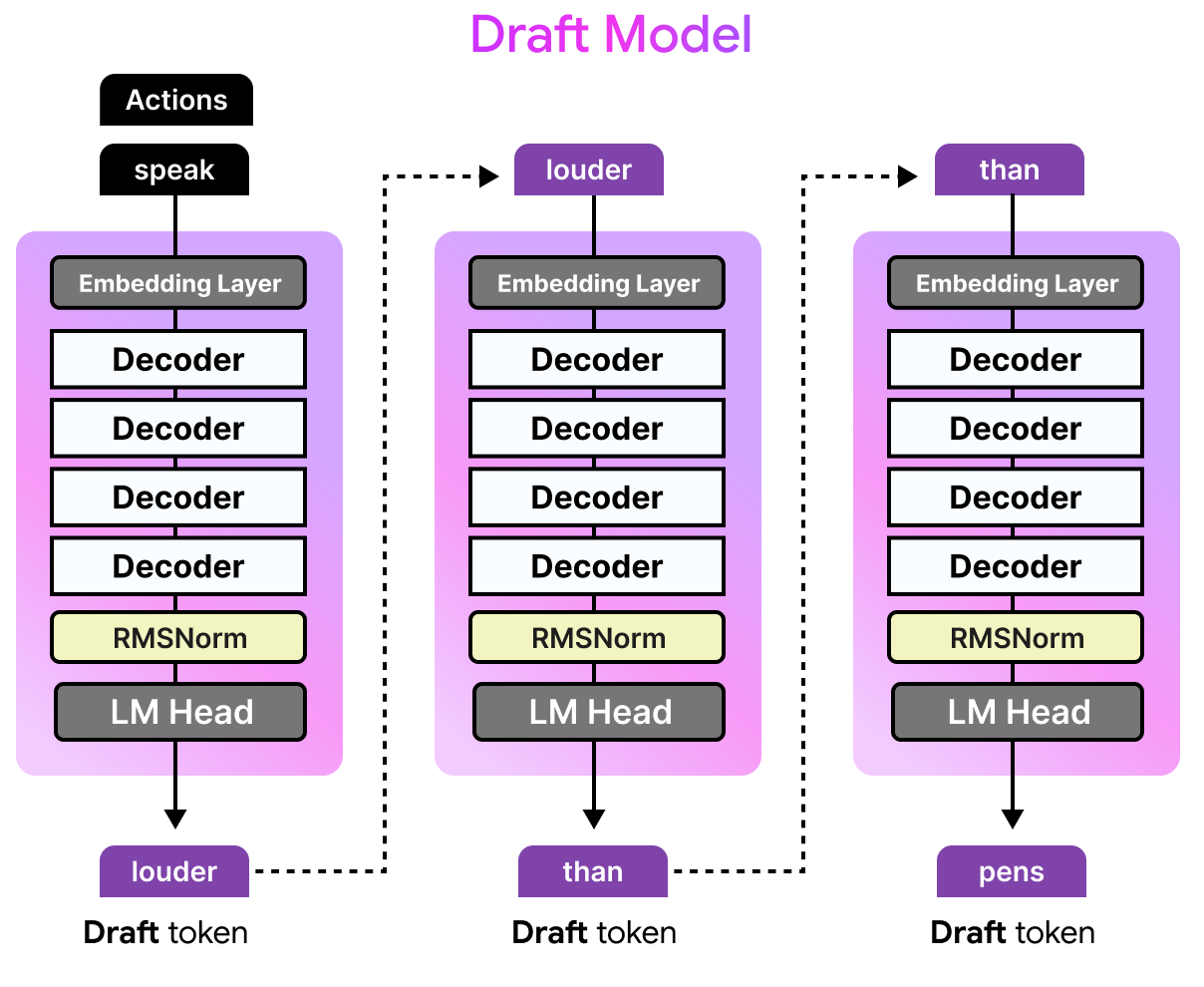
What is Multi-Token Prediction?

However, the drafted tokens are not necessarily correct, otherwise we could just have used the smaller model. Instead, these tokens are given to the target model to verify in parallel. Since the target model can do this in one forward pass, it doesn’t have to do a forward pass for each token. The drafter is what we call the Multi-Token Prediction (MTP) head. Each forward pass of the target model performs regular next-token prediction (NTP) and produces intermediate hidden states. The drafter (MTP Head) uses those hidden states and runs several autoregressive forward passes to general multiple tokens. As such, a single forward pass of the target model results in multiple tokens instead of one. There is one from next-token prediction of the target model and multiple ones from the drafter (MTP head).

If the target model agrees with the suggestions of the draft model, then all tokens are accepted. Instead of having to generate four tokens, the smaller model did that in a fraction of the time. The target model only had to verify them in the time it would have taken the target model to generate one token. Moreover, if all draft tokens were accepted, the target model would still generate one additional token by itself.

If the target model disagrees with only part of the draft tokens, it will accept them until it disagrees. The target model will then replace the rejected token with a token of its own.

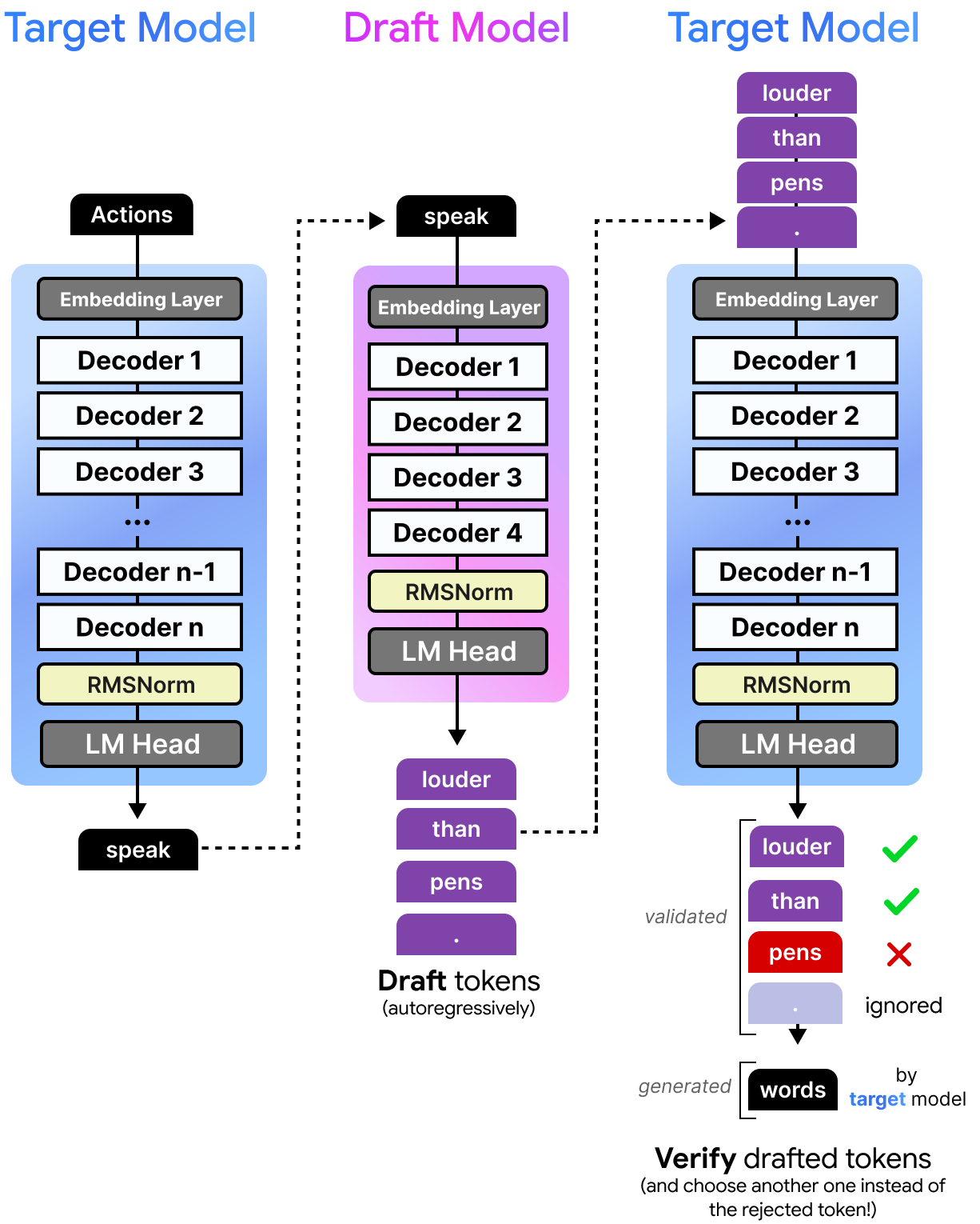
This process is actually quite fast considering the model can verify the quality of the drafted tokens all at once instead of having to verify each of the drafted tokens one at a time. Since the draft model is so small, it takes much less time to predict a single token compared to the target model. This means that the target model can verify multiple tokens at almost the same time it takes to generate a single token! Note that the draft model, like most language models, generates those tokens sequentially but can do this much faster due to its small size.

All tokens that the target model deem to be good enough are selected. The first token it rejects and all others that follow are not included are discarded. However, since the target model has done a forward pass it can still perform a next token prediction. So although a token, like “pens”, is rejected the target model would still come with an alternative of the rejected token.

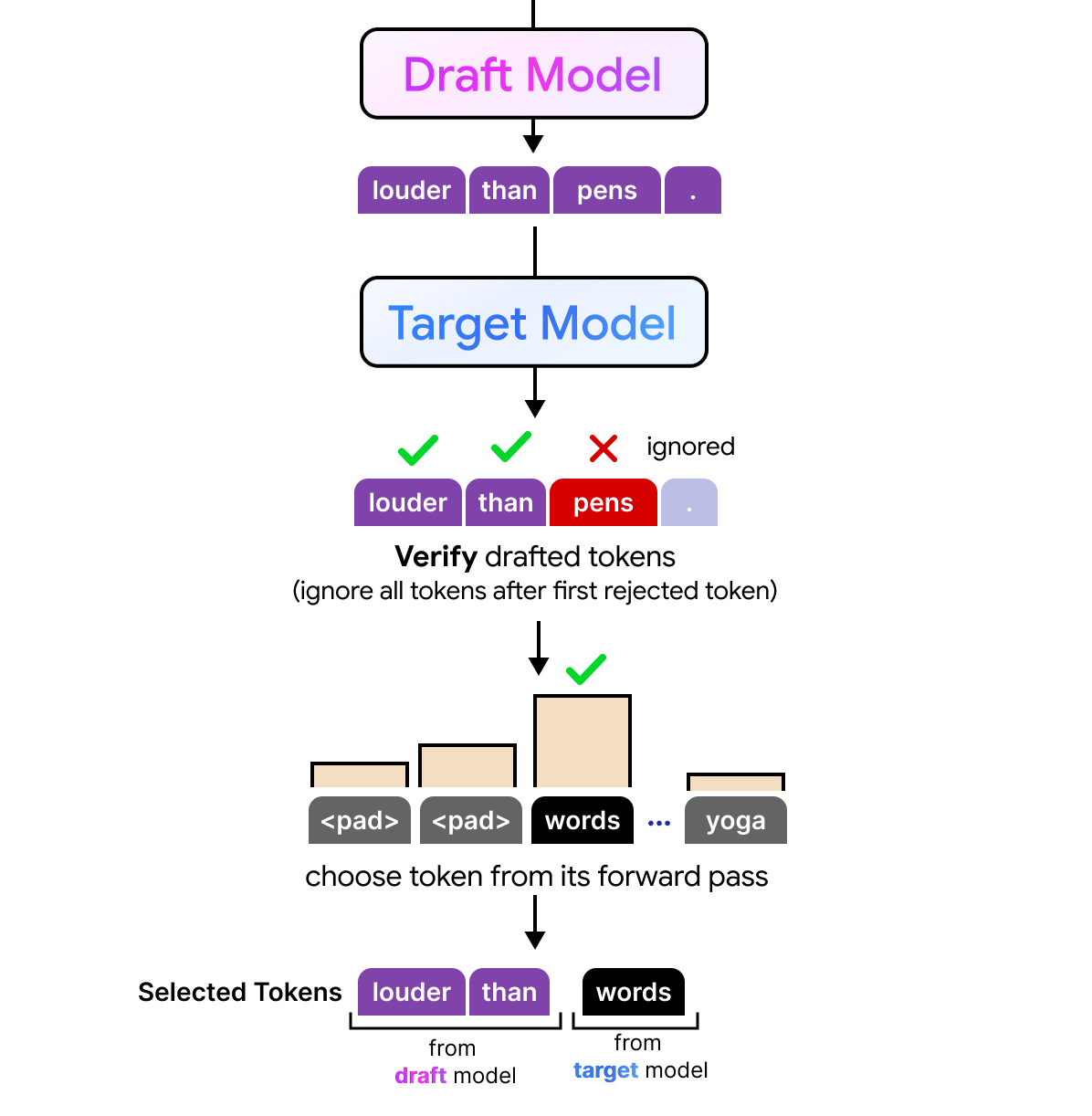
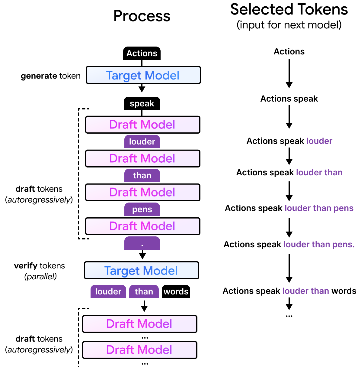
As a result, any number of drafted tokens might be selected by the target model. The full process is quite interesting to visualize considering the draft model performs its processing autoregressively and generates tokens sequence by sequence, the target model can verify all drafted tokens in parallel. The target model is still autoregressive but instead of having to generate those draft tokens one by one, it can now verify them all at once.

MTP with Gemma 4

The draft models released for the Gemma 4 family are most similar to the dense Gemma 4 models, but much much smaller. In fact, the draft model for the Gemma 4 E2B has only about 76M parameters, four layers, and a smaller input embedding size (256 compared to 1536).

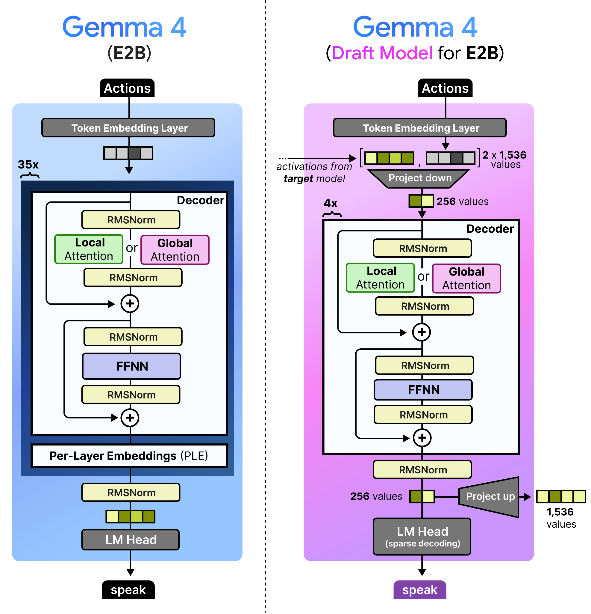
Note how the decoder itself is similar to that of a dense Gemma 4 model. However, there is a lot happening before and after the decoder!

The draft models have various enhancements specifically to make it more efficient and to further speed up inference. Likewise, there are also some interesting techniques used to improve the quality of the drafted tokens and decreases drafter latency. After all, we want the drafted tokens to be as accurate as possible, and to be generated as fast as possible.

These changes can be summarized as follows:

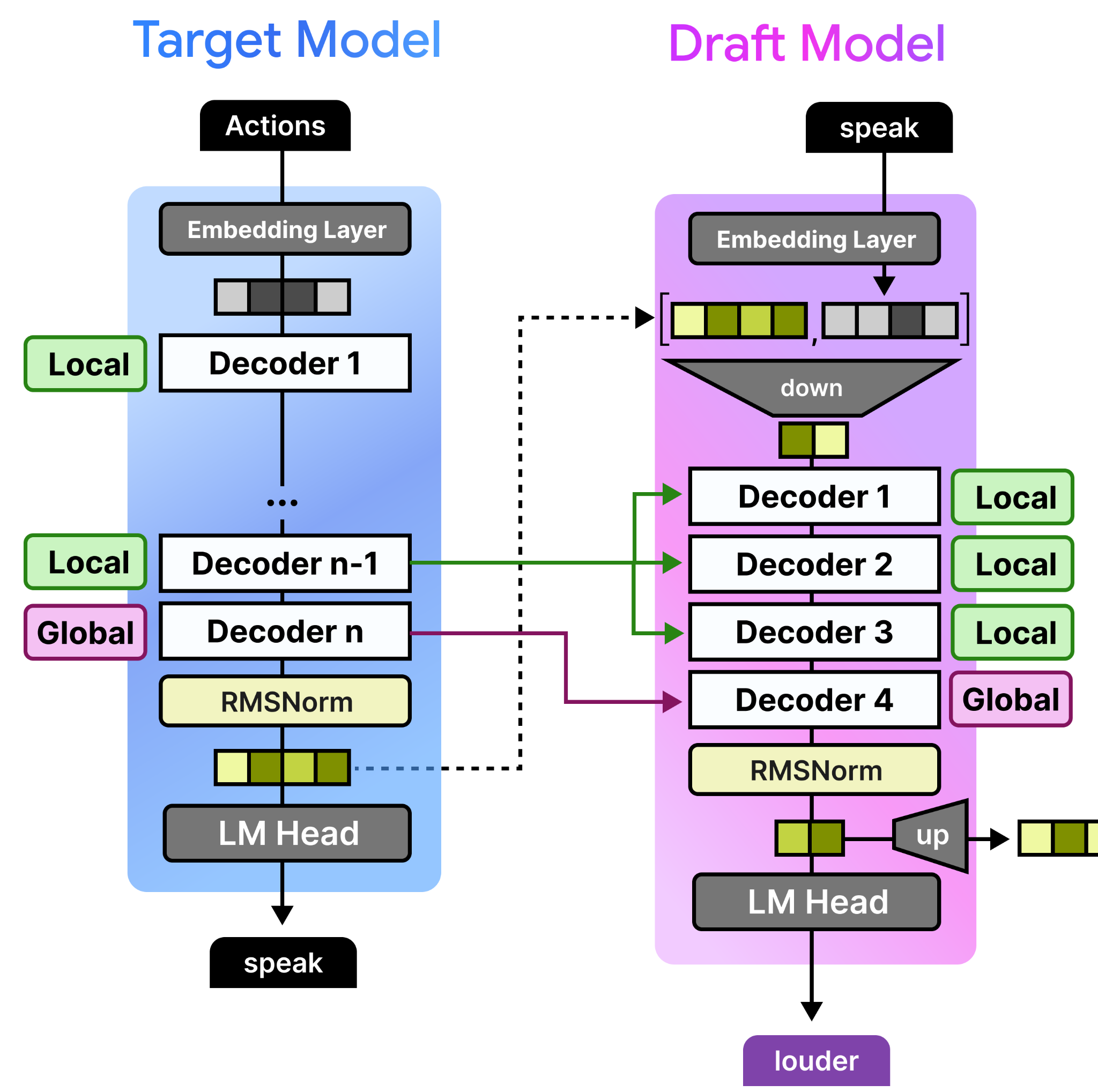
• Target Activations: The draft model uses the activations from the last layer of the target model, concatenates them with the token embeddings, and down-projects them to the drafter model’s dimension.

• KV Cache Sharing: The draft model cross-attends to the target model’s KV cache rather than building its own.

• Efficient Embedder: The LM Head performs a sparse decoding technique that identifies the most likely clusters of tokens to predict (E2B and E4B only).

Let’s explore each of these in more detail!

Target Activations

To improve the quality of the tokens generated by the draft model, the final activations of the target model (e.g., E2B) are fed to the draft model. These are concatenated with the token embedding of the draft model both having 1,536 values assuming the E2B model. The concatenated embeddings are quite large and for efficiency reasons they are projected down to only 256 values. This is essentially a compression of the processed state of the large draft model and the newly initialized embeddings of the draft model. Why let previous activations go to waste?

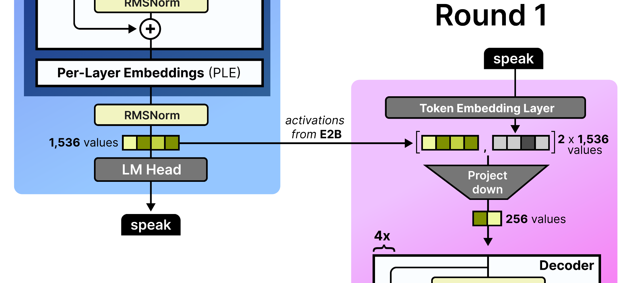
These activations are only given to the draft model in the first round of processing. Remember that after the draft starts with an initial round, it may produce several tokens by passing them back to itself autoregressively. As such, in round 2, the activations that the draft model generated in round 1 are used since a new token was generated. Since the intermediate activations of the small draft model are only 256 values, they are projected up to match the dimensions of its input embedding table (namely 1,536 values). Note that to further improve efficiency, the input embedding table is shared between the target model and the draft model.

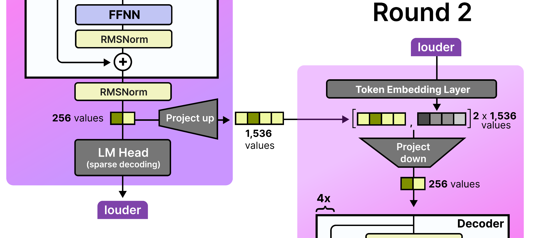
Then, in round 3, the draft model uses the activations that were generated in round 2, and so on!

KV Cache Sharing

The KV cache can take up quite a bit of space since it contains the key and value representations for every token in the sequence, across every layer. Although Gemma 4 has already taken many steps to reduce this (like setting K=V in the global attention layer), the draft model takes it a step further.

Instead of the draft model needing to process the full prompt and build its own KV cache, it cross-attends to the already-computed KV cache of the target model. For its local attention layers, the draft model simply reuses the last computed local KV cache of the target model. Since the last layer of any Gemma 4 model is always global, that global KV cache is reused for the draft model’s global attention layer.

As before, since the target model already did much of the heavy lifting, it would be a waste to throw that away!

The Efficient Embedder

Finally, there is an efficient embedder that reduces the compute needed to generate the drafted tokens from the Language Model Head (LM Head). In traditional models, the LM Head would convert the hidden state generated by the decoders to logits (token probabilities) by multiplying it with a large weights matrix (the same used in the embedding layer, namely the lookup table). For such a small model, this process can be quite expensive!

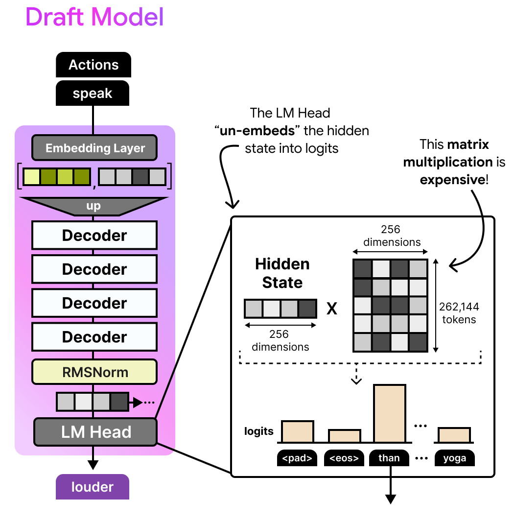
The question you might ask yourself is whether we really need to calculate the logits for all 262,144 tokens when most of them are likely to be irrelevant?

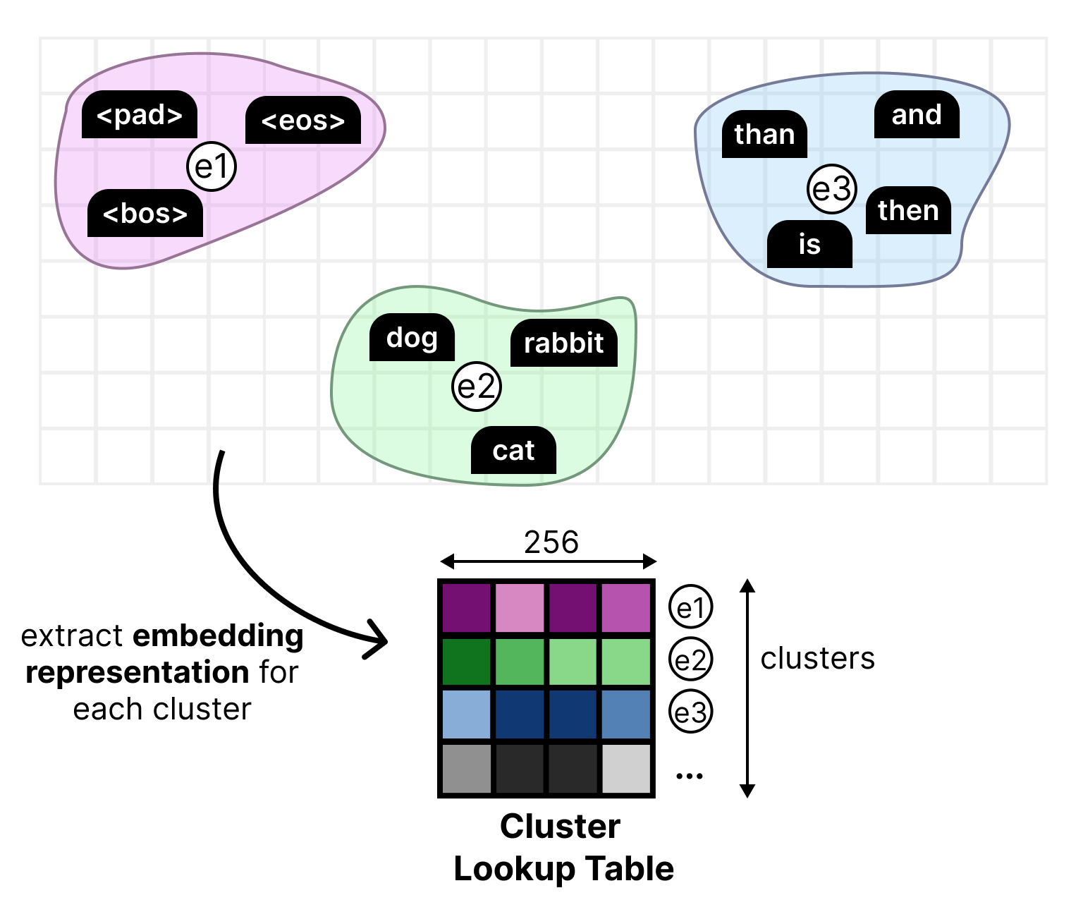
In the drafter for Gemma 4 E2B and E4B models, this process is made more efficient through a classic technique, namely clustering. All token embeddings have been clustered separately into large groups of tokens that have similar meaning. We then find an embedding representation for each cluster.

This new lookup table is then used in the LM Head where it is multiplied by the hidden state. This results in cluster logits instead of token logits. This means that the cluster logits tell us the clusters that most likely contain the next token. The clusters that are most likely to contain the correct token are selected. Then, all tokens within those clusters are used to calculate the final token logits.

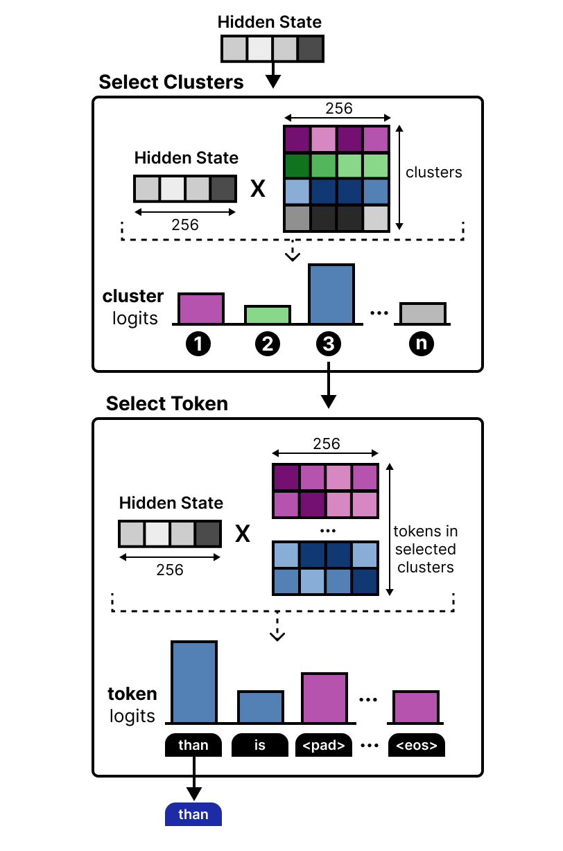
This computation is much easier and instead tells us that the next token is almost certainly in the chosen clusters. This efficient embedder allows for speeding up the draft model even more!

My First Weeks at Google DeepMind

It’s now been about 8 weeks (almost 2 months already!) since I started at Google DeepMind and what a rollercoaster it has been. Building in public and sharing with the public has been a passion of mine so it’s been an absolute pleasure to work on this launch!

I’m grateful to a lot of people that gave feedback on this visual guide: Edouard Yvinec, Lucas Dixon, Sabela Ramos, Omri Homburger, Filippo Galgani, Tatiana Matejovicova, Lawrence Stewart, Petar Veličković, Federico Barbero, Alice Coucke, Tal Schuster, Johan Ferret, Utku Evci, Shreya Pathak, Ziwei Ji, Ivan Korotkov, and everyone that I might have forgotten ;)

I worked on this during my onboarding whilst also preparing for this release, so I wouldn’t be surprised if any mistakes slipped in during the chaos. If it did, please let me know!

…

Now that you made it to the end, I’m curious… What do you all think about me doing this more? Should I convince my manager to continue doing this kind of content?