
A Visual Guide to DiffusionGemma
Going beyond autoregression.

Following the release of Gemma 4 12B there is yet another innovative model that I can introduce to you all, DiffusionGemma!
This is one I’m especially excited about because it’s a different way of approaching text generation, yet uses many of the great things we have with existing “regular” LLMs. We are going to explore the old, the new, and how they live side-by-side.
In this guide, I’m going through a lot of things because there is so much that makes DiffusionGemma special! You will learn more about diffusion in general, how it works for discrete text, the architecture of DiffusionGemma, and all of the interesting techniques used.
Get ready, this is going to be a fun one to explore ;)
The Problem with Autoregressive Models
Autoregressive Large Language Models generate one token at a time and are great for serving many users at once. Why? Because generating a single token for a single user is surprisingly cheap in terms of computation. In each step, a significant portion of the time to generate a token is spent loading the weights from memory and not the actual computing.
During decoding, these regular Transformer models are memory bound rather than compute bound. This means that, for instance, the time it takes to generate one token is the same for one user as it is for 256 users.
The reason for this is that the weights only need to be loaded from memory once per step, regardless of how many users are being served. This means that whether we multiply those weights against 1 user’s vector or those of 256 users, the cost of moving the weights into memory stays the same. By batching all users together, we get the same amount of work for nearly the same cost.
This is not a free lunch though, after a certain point (which depends on the chip itself), the LLM might be serving too many users and lacks compute instead. You can visualize this tradeoff with a roofline plot. It shows the impact of increasing the chip’s performance (how long it needs to spend to generate a token) versus the chip’s memory (how fast it can load data from memory).
When only serving one user (batch size of 1), the LLM is memory-bound and loads a large number of weights without actually doing much computation. The more we increase the batch size (same memory load but more computation), you approach a “ride point” where the hardware is properly utilized.
Thus, while batching is great for serving many users at once, there is nothing to be gained for the individual user! It still receives their tokens with the same speed. No difference in latency.
DiffusionGemma flips the script.
What if we used the compute’s idle time for a single user instead? Instead of generating 1 token each for 256 users, what if we generated 256 tokens at once for 1 user?
This is the core idea behind DiffusionGemma! The model starts with a sequence of 256 randomly initialized tokens (called a canvas) and tries to choose better tokens for the entire canvas all at the same time. By predicting 256 tokens at the same time, the compute budget of 256 tokens is now focused on a single user instead of spreading it across many users.
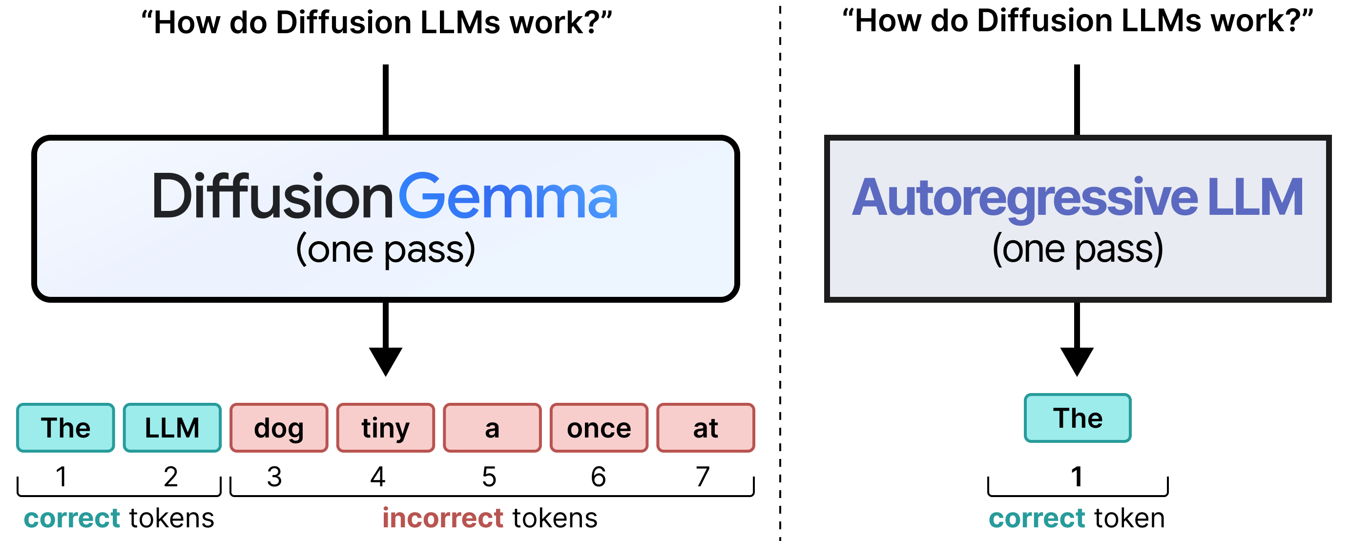
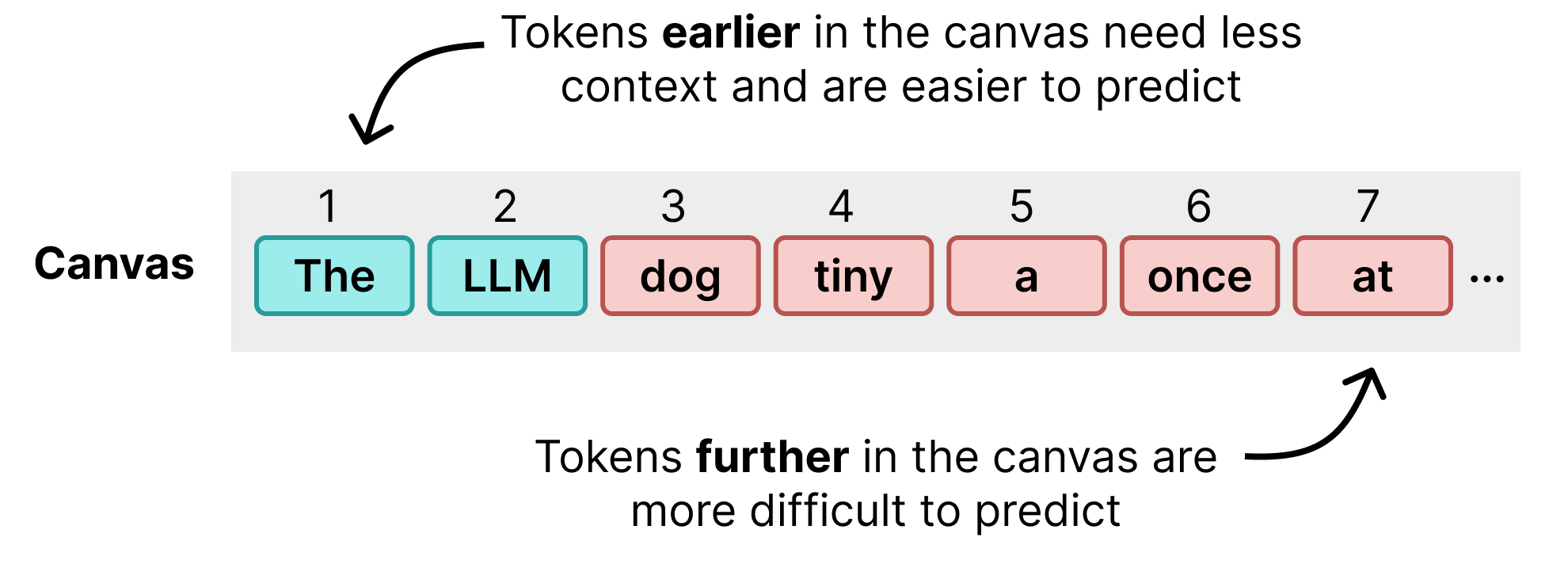
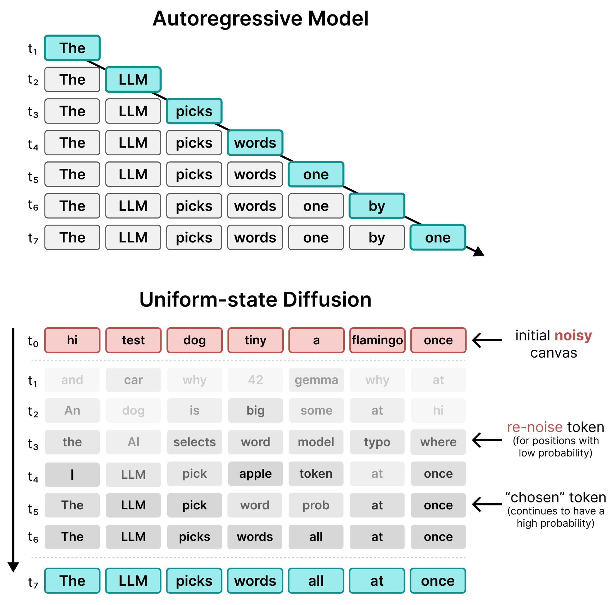
Of course, predicting so many tokens at once is very difficult and the model will have a hard time predicting token 254 without knowing which tokens came before it. Note how the first two tokens are great but it slowly starts to output nonsense. A first pass of DiffusionGemma on this canvas tends to produce reasonably accurate tokens at the start of the canvas but poor ones towards the end.
So instead of doing a single pass, what happens if we simply perform multiple passes?
This is where iterative refinement comes in. The model takes another pass over the canvas using its previous predictions. Correct tokens (those that still have high probabilities) help the model make better guesses further into the canvas. With each pass, the model improves tokens that previously had low probabilities or were surrounded by inaccurate tokens. After a number of iterations, the canvas then converges to a text of similar quality to that of regular Transformer models, just much much faster for a single user. The main reason for this is that the model does much fewer forward passes than the number of tokens it generates.
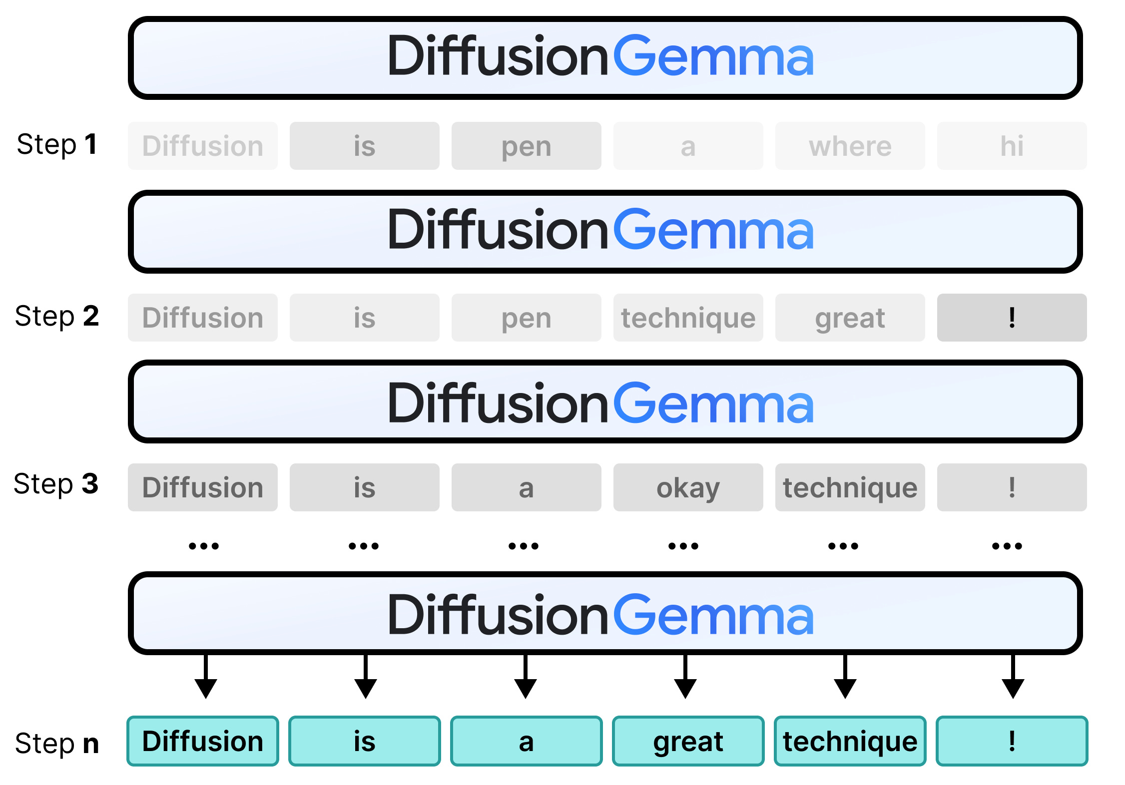
See how we just went from next-token prediction on regular Transformer models to 256 tokens all at once!
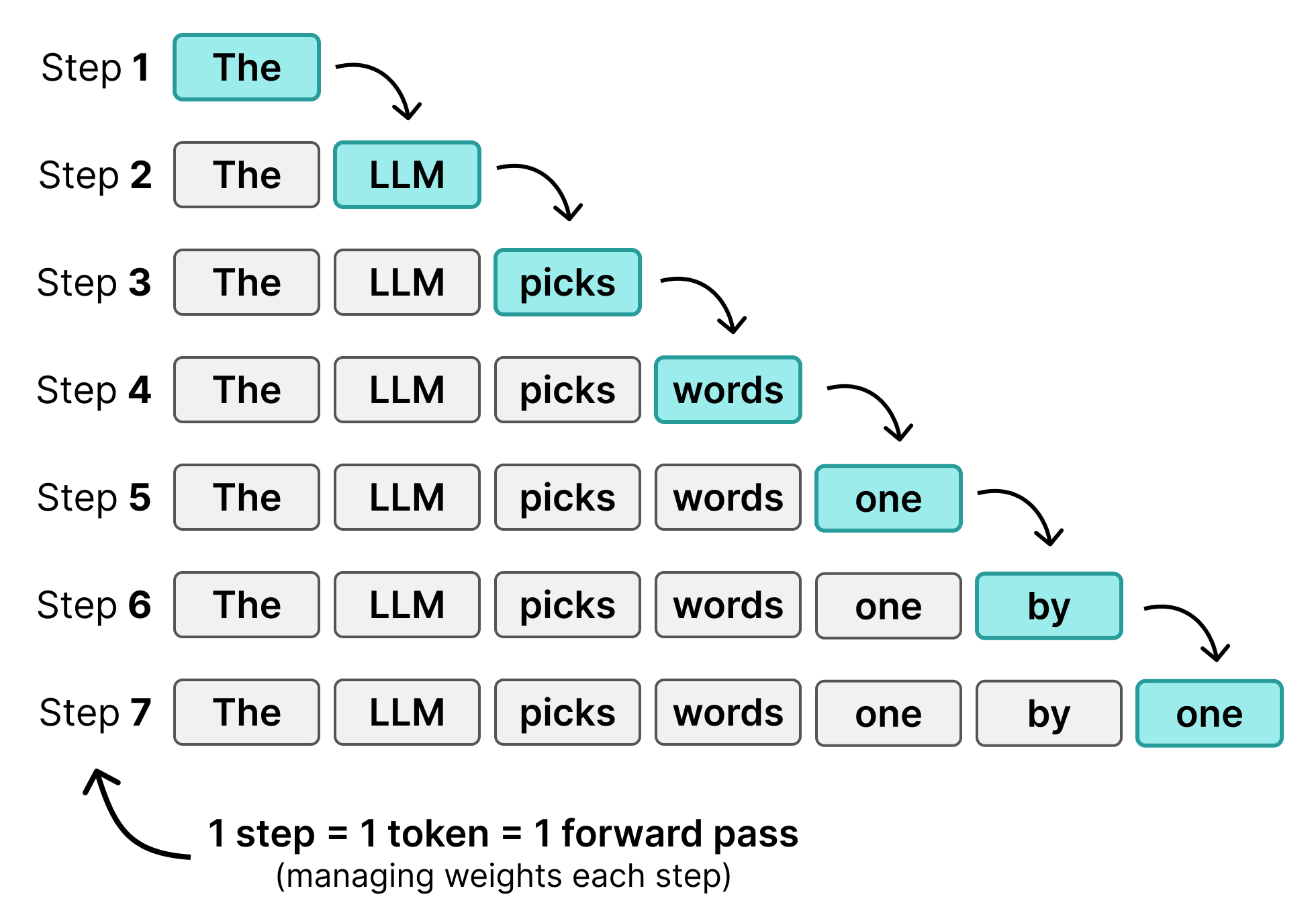
Although both use a number of steps to generate the output, a regular Transformer uses one step per token whilst DiffusionGemma uses each step to improve upon a canvas. What makes this possible is a technique called diffusion which became popular in the field of image generation. It is closely related to the concept of iterative refinement.
Instead of the model being memory-bound (like the Autoregressive LLM), the Diffusion LLM is compute-bound instead and scales more quickly as you add more compute.
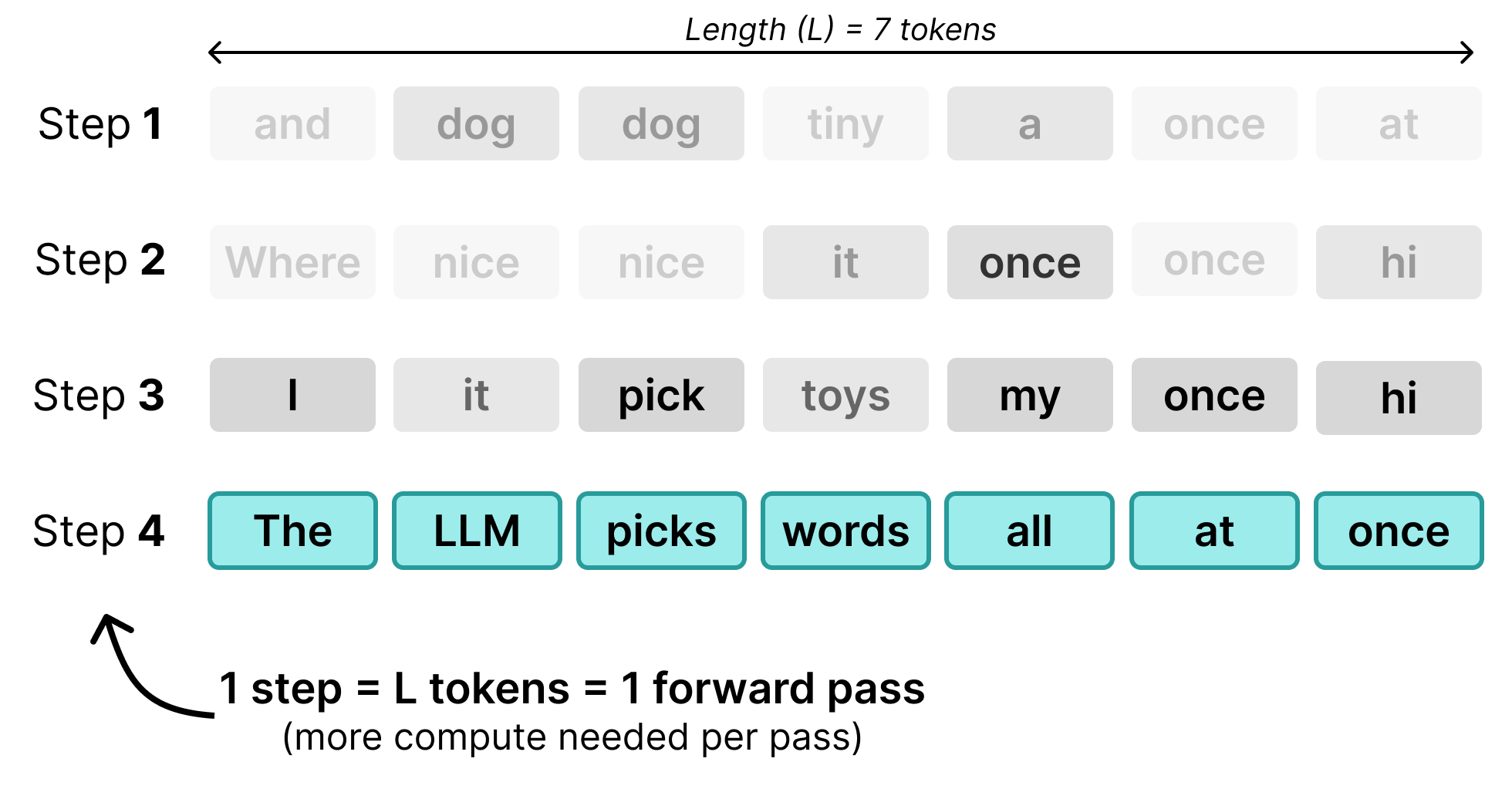
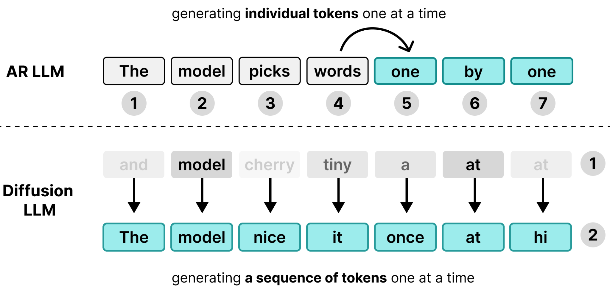
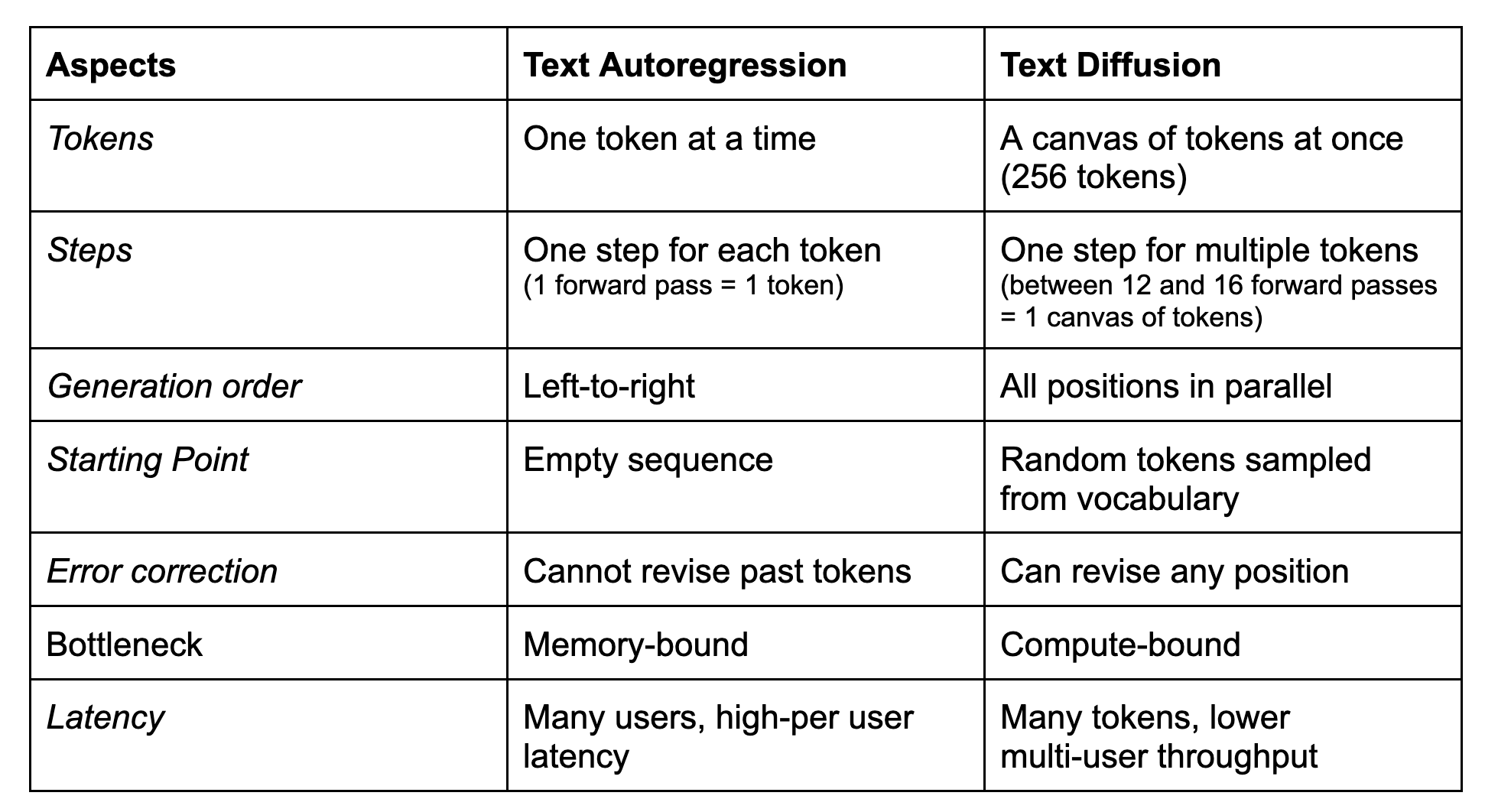
What you get is the main difference between Autoregressive and Diffusion LLMs, namely the way they process the same tokens. Autoregressive LLMs generate one token each forward pass and are memory-bound when serving a single user whereas Diffusion LLMs generate a sequence of tokens each forward pass and are compute-bound.
So let’s explore diffusion in more detail and how DiffusionGemma took that principle for image generation and applied it to text generation.
What is Diffusion?
Diffusion is a process in image generation which centers around “noise”.
Diffusion for Images
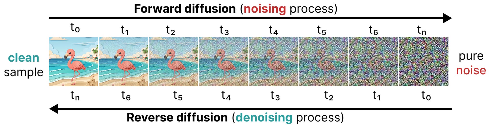
Diffusion is a process in image generation which centers around removing “noise” from an image. Starting with a randomly initialized image (100% “noise”), diffusion attempts to reduce the amount of noise with each subsequent step. In image generation, this process is guided by a prompt. After enough steps, it will eventually generate or “uncover” an image.
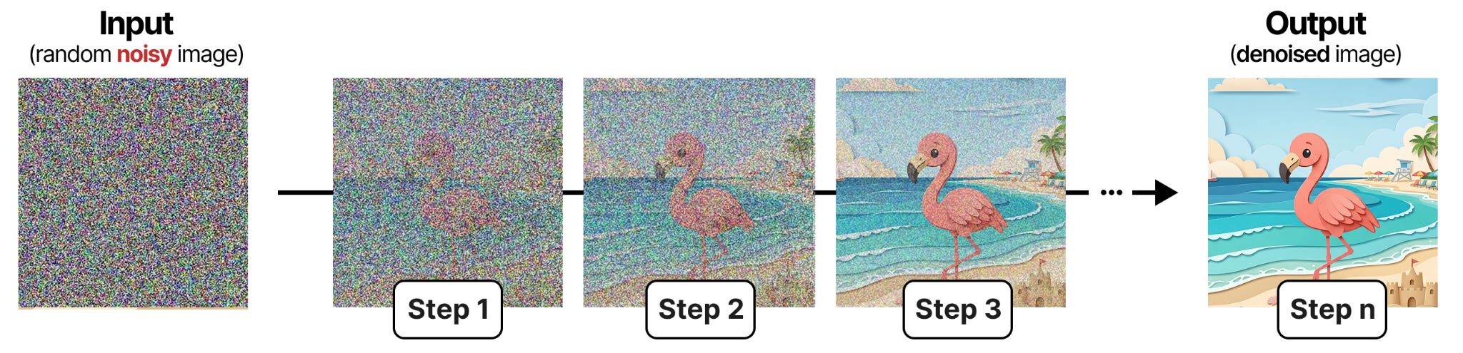
The process of reducing the amount of noise in an image is called denoising. As you can see from the figure, this is an iterative and sequential process. With each step, you can see the image a little bit better and by the end, the full image is shown. This principle is not only central to image diffusion but as you will see, also to DiffusionGemma.
This process of denoising is guided by two main principles, forward diffusion and reverse diffusion.
Forward Diffusion
To have the model learn how to denoise an image, you will have to start with some training data. This data contains image/text pairs. For each pair, you add a certain amount of random (Gaussian) noise to the image.
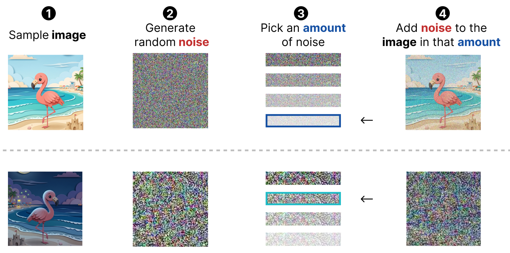
This process is called forward diffusion. It creates new data from existing data and adds a signal to the training process.
Reverse Diffusion
Reverse Diffusion, on the other hand, attempts to train a model to predict the noise we added to the initial data. This training data then has a clear signal to predict: the noise. You are essentially telling the model, here is a noisy image and from that I want you to only predict the noise.
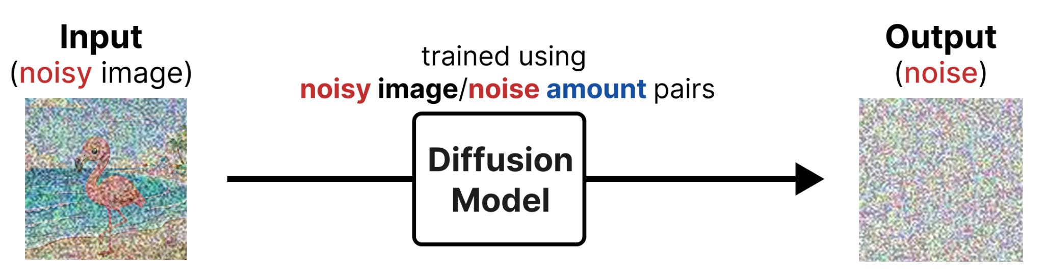
So why would we want to introduce noise into the images and then attempt to predict it?
Well, we can subtract the predicted noise from the noisy image to get it closer to the images that the model was trained on. By doing this iteratively, you can start with complete noise and slowly denoise it until there is no more noise left in the image.
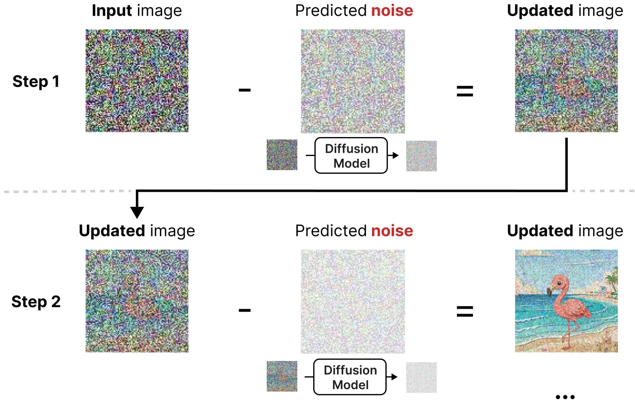
Together, forward diffusion (generating noisy training data) and reverse diffusion (denoising noisy input data) create this process of breaking and fixing an image.
Note that in image diffusion this process is guided by a prompt which serves as an extra signal to decide what is and what isn’t noise. Without something to guide it, the model has no idea what it should create in the first place.
What guides this process is called the encoder and serves to process the input query and understand the semantic meaning behind it. The output of the encoder is then passed to the diffusion model so it is guided to create the image in your query. Without the encoder, the diffusion model would have no idea what to create from the 100% noise it receives at the first step.
Together, they create the full pipeline which consists of two main architectures:
Denoiser – The model used to iteratively remove noise from the noisy input (e.g., a diffusion model).
Encoder – The model used to process the input query (e.g., an encoder language model).
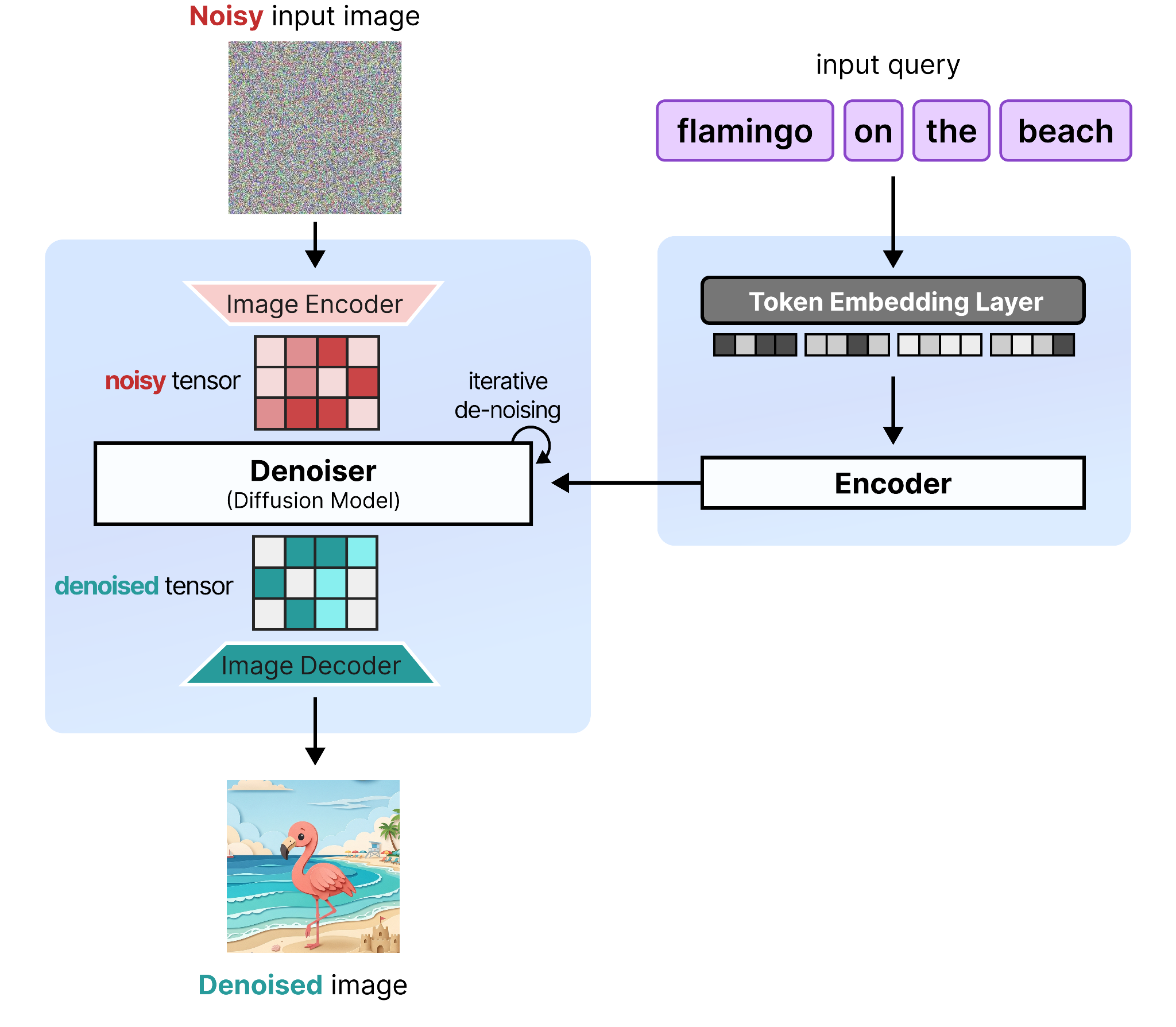
As shown before, the diffusion model is also called the denoiser since it focuses primarily on removing noise from a noisy input. We are going to be using this term throughout to showcase the purpose of the model.
Diffusion for Text
Now that we have seen diffusion for images, how can that be translated to text? It is easier to add individual noise to pixels as those are continuous values. You can make a red pixel a little bit less red and a little bit more blue. However, how do you make the token “The” a little bit less “The”? What constitutes “noise” for a single token?
Masked Diffusion
Instead of looking at them as individual tokens, let’s consider the whole. In masked language modeling, like is done when training encoder models like BERT, random tokens in the input are replaced with the [MASK] token. We can consider this [MASK] token to be “noise” (also called corrupted tokens).
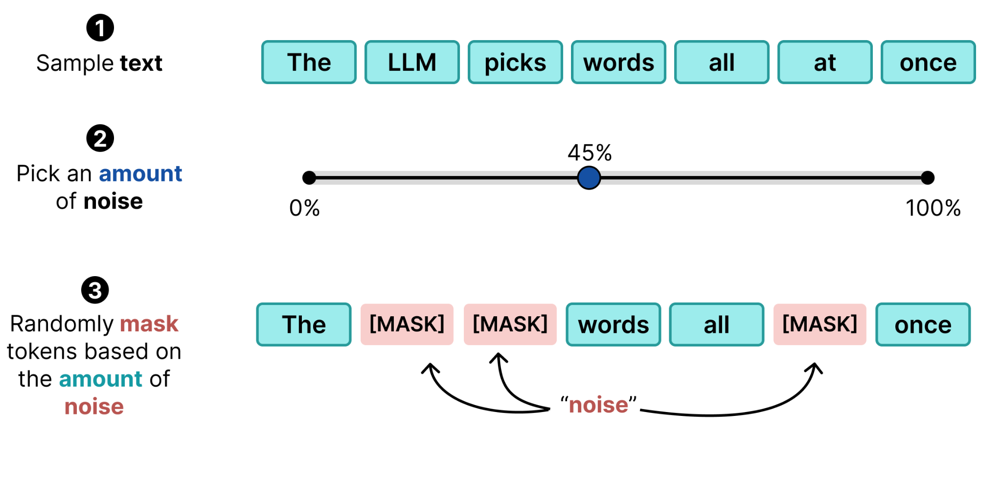
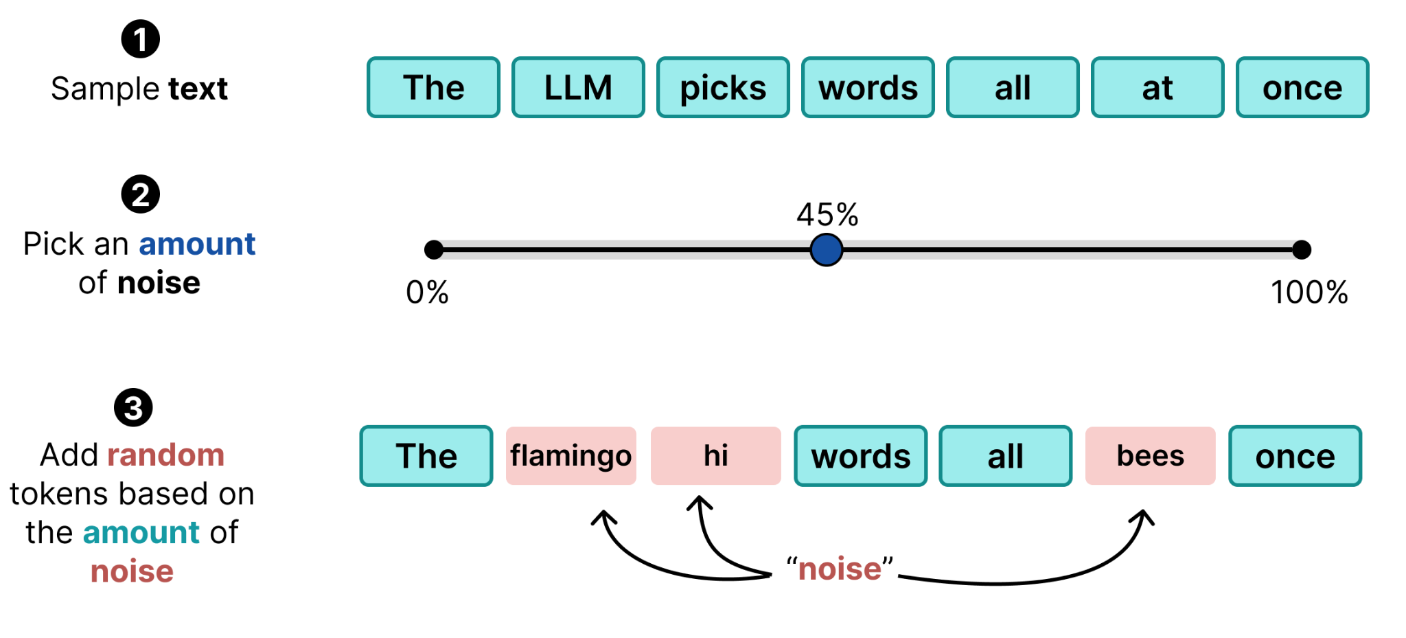
The procedure then becomes similar to what we have seen in Diffusion for Images, you sample a given text, pick an amount of noise, and randomly mask tokens based on the amount of noise.
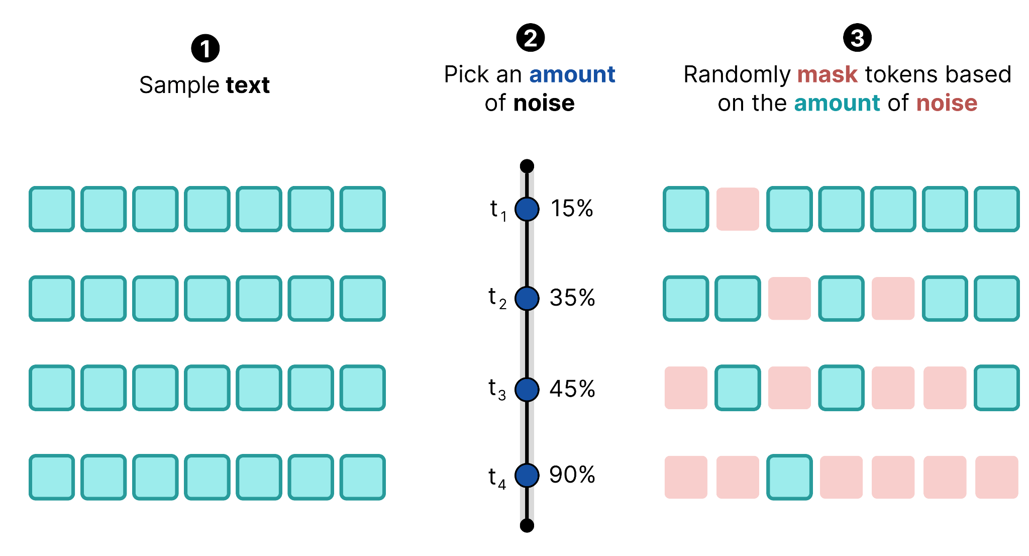
When we do this multiple times, we can create a training dataset. You sample the same text (or different ones) and add different amounts of noise. This allows the model to learn how to denoise different amounts of noise, just like with Diffusion for images.
This forward diffusion process is then followed by reverse diffusion, which would have the model predict what the correct token should be at the [MASK] position. At each step, the model denoises only the tokens for which it is confident it has a good replacement.
During a single denoising step, the model predicts the most probable token at each canvas position. Then, only the tokens that exceed a certain threshold will get chosen. The ones that do not meet the threshold will remain a masked token.
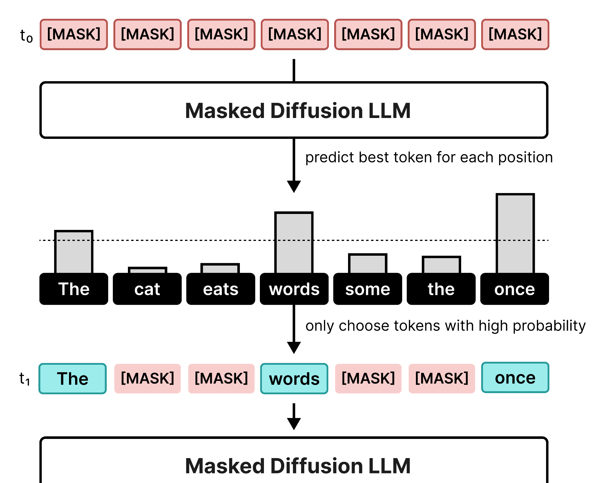
This process continues until all masked tokens are replaced or until a certain number of steps are reached. Generally, the more steps you use the more accurate the resulting sequence will be. Instead of coming to all tokens at once, it can use several steps to decide which tokens should go where.
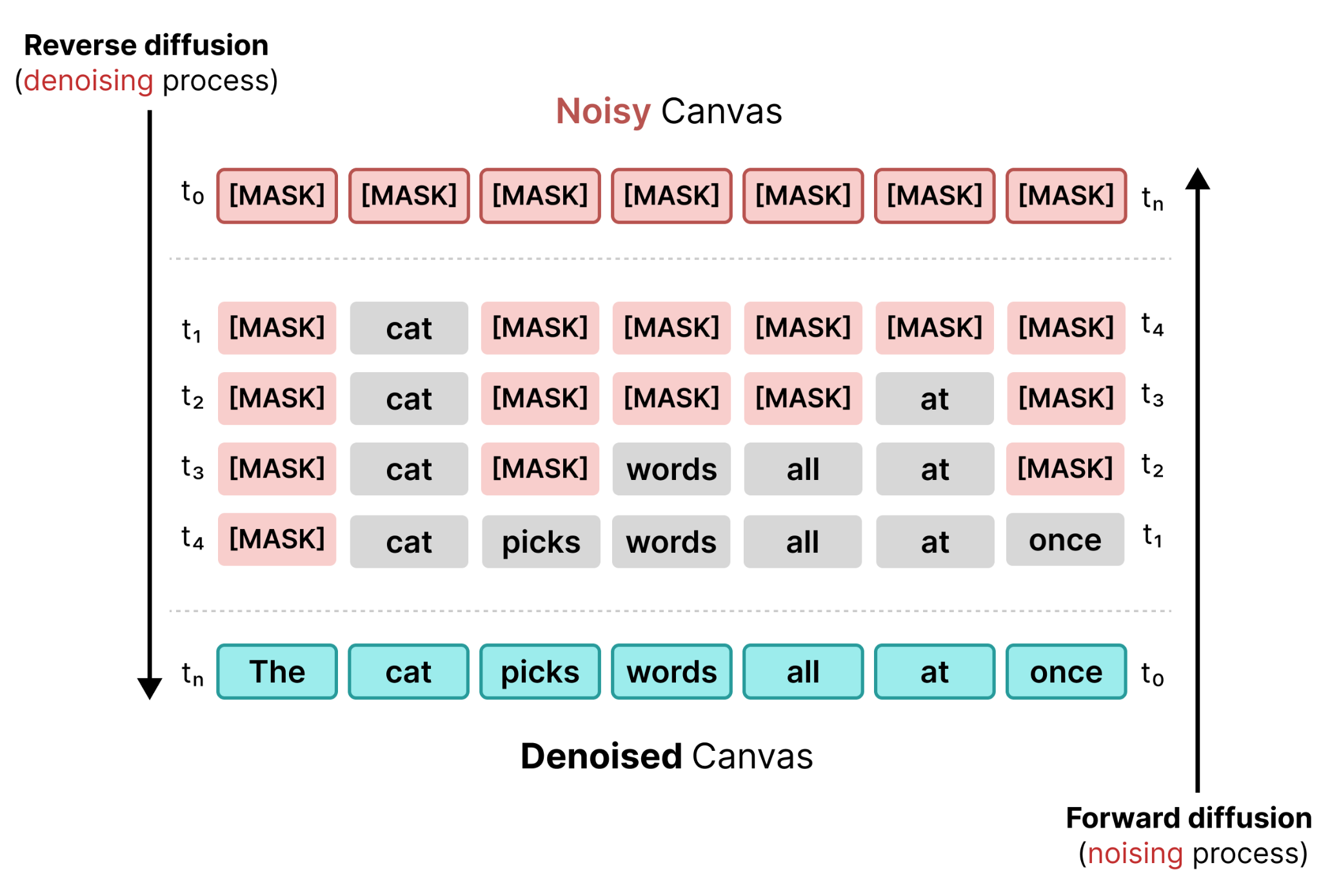
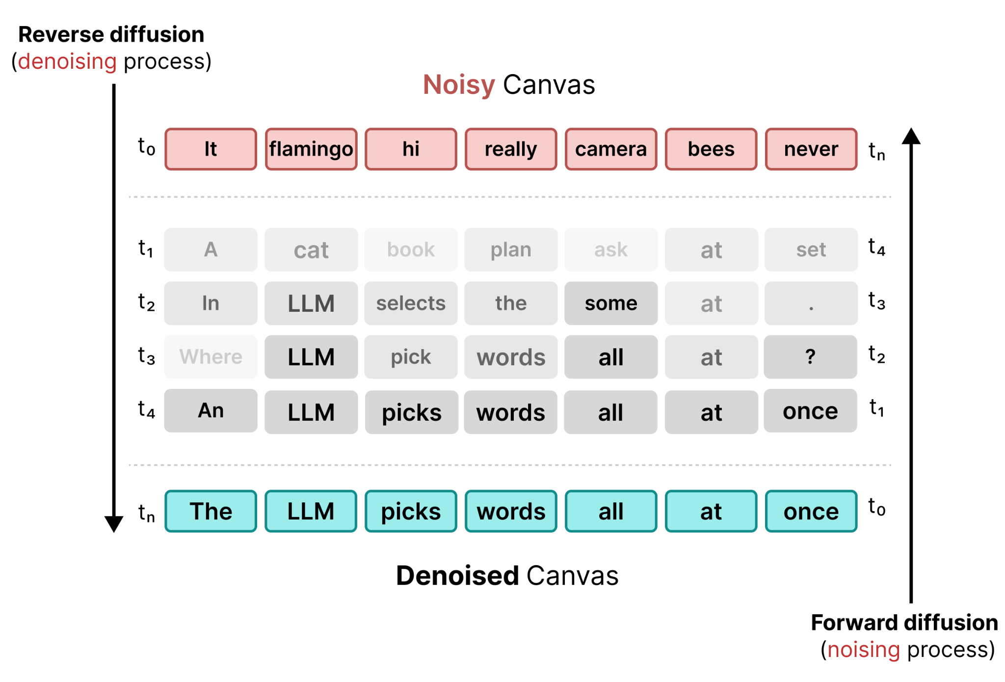
Like with Diffusion for images, we can visualize the forward and reverse masked diffusion process in one figure:
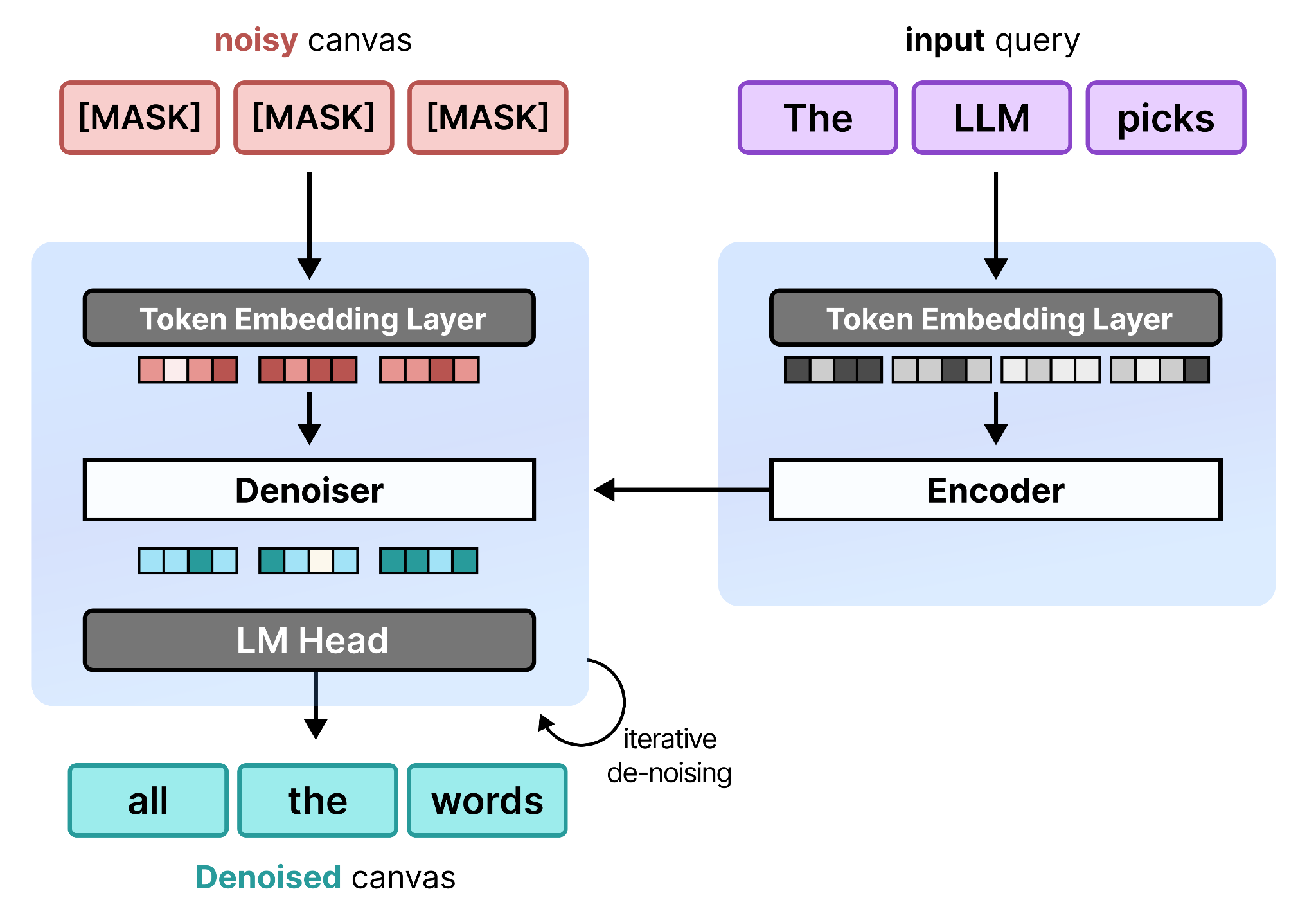
Much like diffusion for image, diffusion for text generally consists of two models (or two techniques) used in conjunction:
Denoiser – The model used to iteratively remove noise from the noisy input (more on this in the “Architecture of DiffusionGemma” section)
Encoder – The model used to process the input query (e.g., an encoder language model).
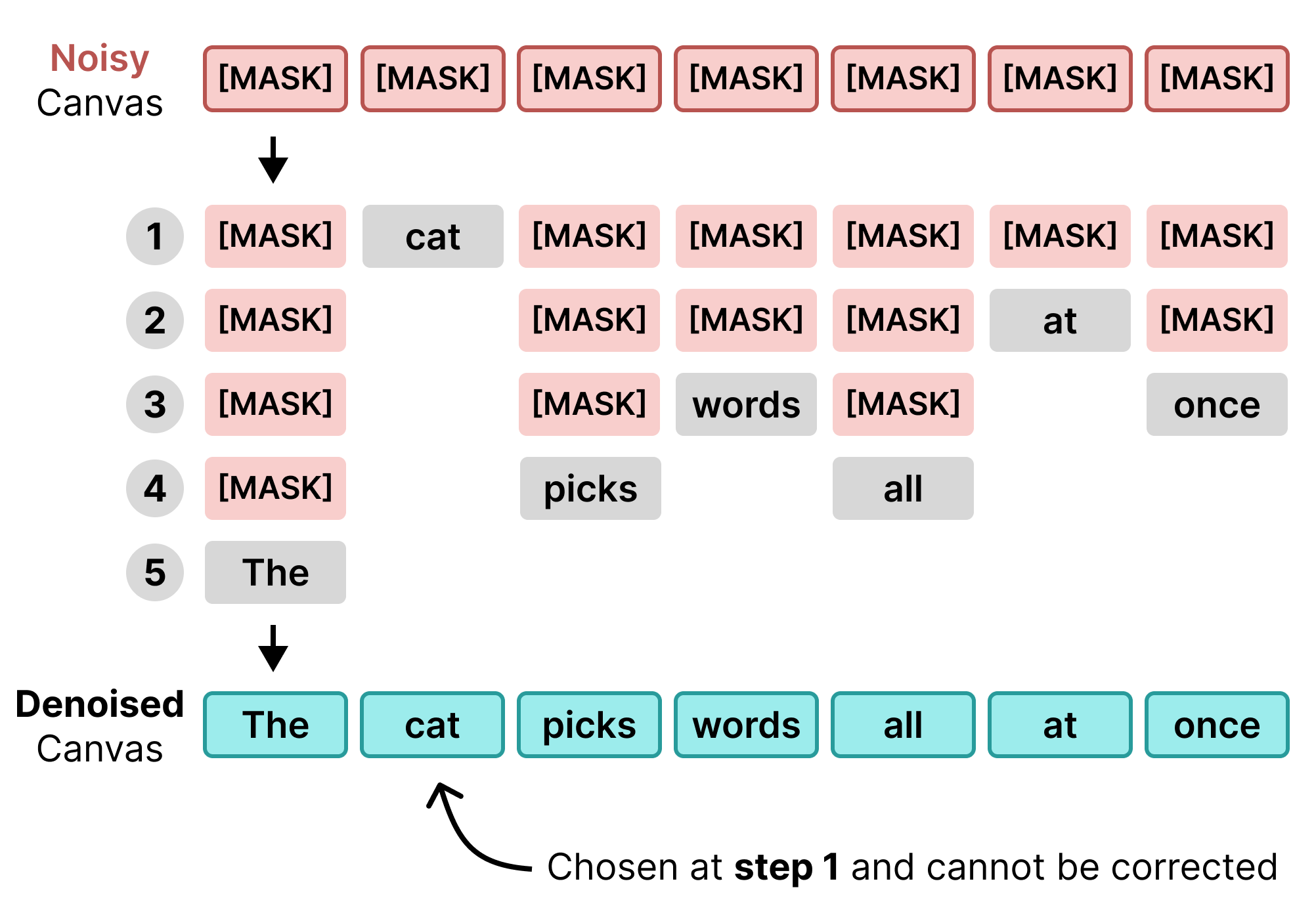
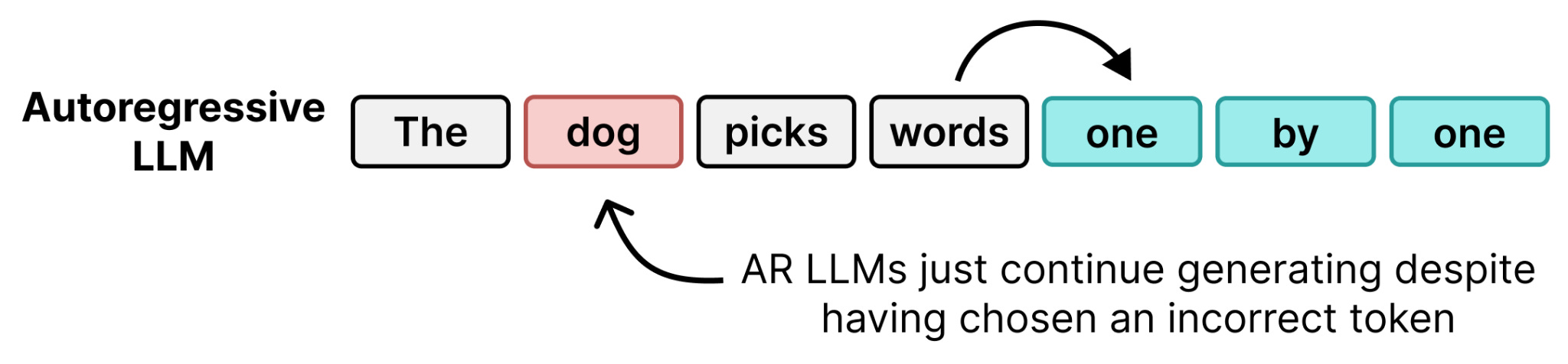
There is one problem though with masked diffusion and that is self-correction! Whenever the model decides to replace a [MASK] token, it is fixed. Once chosen it cannot be replaced. This hinders its potential to correct some of the tokens it might have chosen too early. It is actually similar behavior to autoregressive models that likewise choose a token and are “stuck” with the selected token.
Instead, what if we were to explore a different type of “noise” instead?
Uniform State Diffusion
Using a [MASK] token is a rather “strict” form of defining noise. It either is there or it isn’t, with nothing in between. When compared with image diffusion this is a rather “boolean” way of looking at text. Moreover, when a token is selected to replace a given [MASK] token, it cannot be replaced again.
Instead of corrupting a sequence of tokens by replacing them with the same thing (a [MASK] token) we can replace each token with something different (a random token). In the forward diffusion process, random tokens are used as noise to create a dataset the same way you would do with masked diffusion.
This process creates a dataset with noise but without making it explicit where the noise is (aside from having the ground truth). What makes this so different from masking is that the model has to figure out where the noise is coming from and adjust accordingly. Whether there is 10% of replaced words or 90% requires a thorough understanding of the input.
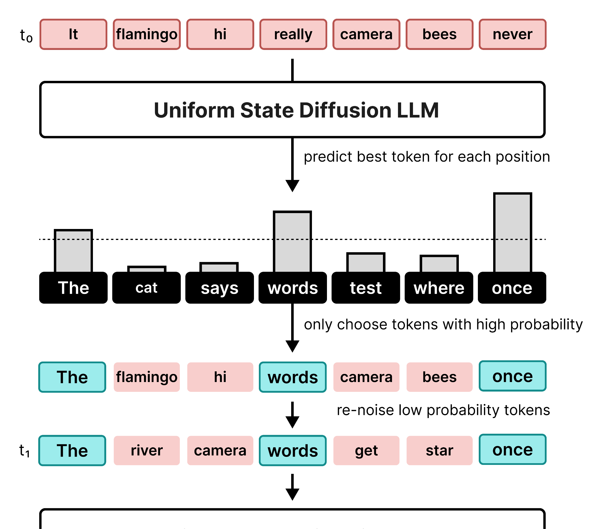
In the denoising process (reverse diffusion), the model has to detect which tokens are noise and which should be updated. At each denoising step, the model predicts a token for each location in the canvas. If a token shouldn’t change, it will keep the high probability. However, if it decides to replace that token, another token with a high probability will be generated instead. As such, the model continues to predict the best token for each position. This also means that a token that might have gotten a high probability in steps 1 through 10 might suddenly get a low probability in step 11 as the canvas gets updated.
Therefore, at each position in the canvas, the model suggests a token with a certain probability. If it reaches a certain threshold, it will be put in that position. However, if it does not meet the threshold, the tokens that were there previously will be re-noised and replaced with a random token.
So why would you re-noise low probability tokens?
If you kept the old token, then that wouldn’t be a uniformly random token. The model has learned during training that the canvas would consist of partially noised tokens that were drawn following a uniform distribution. By keeping the old one, the model might start planning around the wrong token in the next step. To stay close to the training data, and for practical reasons, you re-noise low probability tokens.
Together, forward diffusion (generating noisy text sequences) and reverse diffusion (denoising random tokens) create this process of breaking and fixing a sequence of tokens.
As a result, the model does not stop when it replaces a random token with another token. It can still change any token in the canvas. Compared to Masked Diffusion, this allows the model to continuously update and change the canvas as it goes through steps.
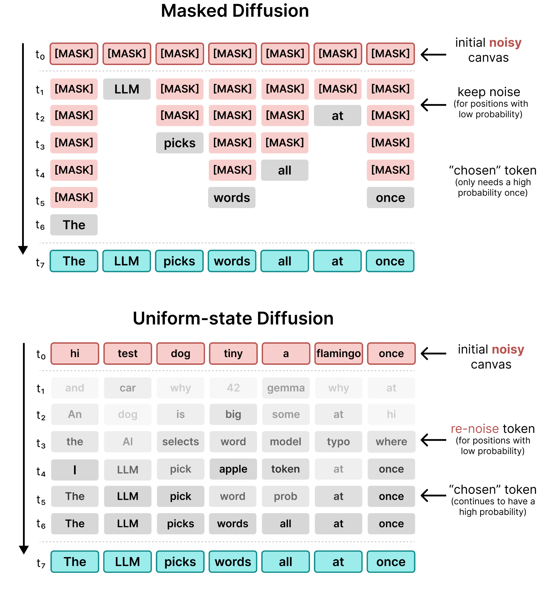
Uniform-state diffusion, and text-based diffusion in general, as such is quite different from autoregressive models. Where autoregression is predicting one token at a time sequentially, diffusion iteratively updates a canvas. This difference between autoregression and diffusion is especially pronounced when we put them side-by-side.
These differences are important because they help you understand when you might choose a text diffusion model over an autoregressive one and vice versa. Although text diffusion models excel at generating many tokens for a single user, they have lower multi-user throughput than their autoregressive counterparts. As such, there is no free lunch with text diffusion. Here’s an overview of some of the fundamental differences between them:
One downside to note of text diffusion, and uniform state diffusion in particular, is that they are difficult to train. The reason for that is that the training objective does not only need to denoise canvases at various noise levels, it also needs to first identify which tokens are actually noise in the first place. Otherwise, it would just consider all tokens in the canvas to be noise, which is not ideal.
So how can we have the benefits of Uniform State Diffusion without the downsides of training? Let’s explore the solution in the Encoder-Decoder patch of DiffusionGemma!
Architecture of DiffusionGemma
DiffusionGemma applies Uniform State Diffusion that we explore thus far. However, the downsides of training this entirely from scratch still remains. The solution was simply not to train from scratch but to use an existing checkpoint as a start instead, namely the Gemma 4 26B A4B model.
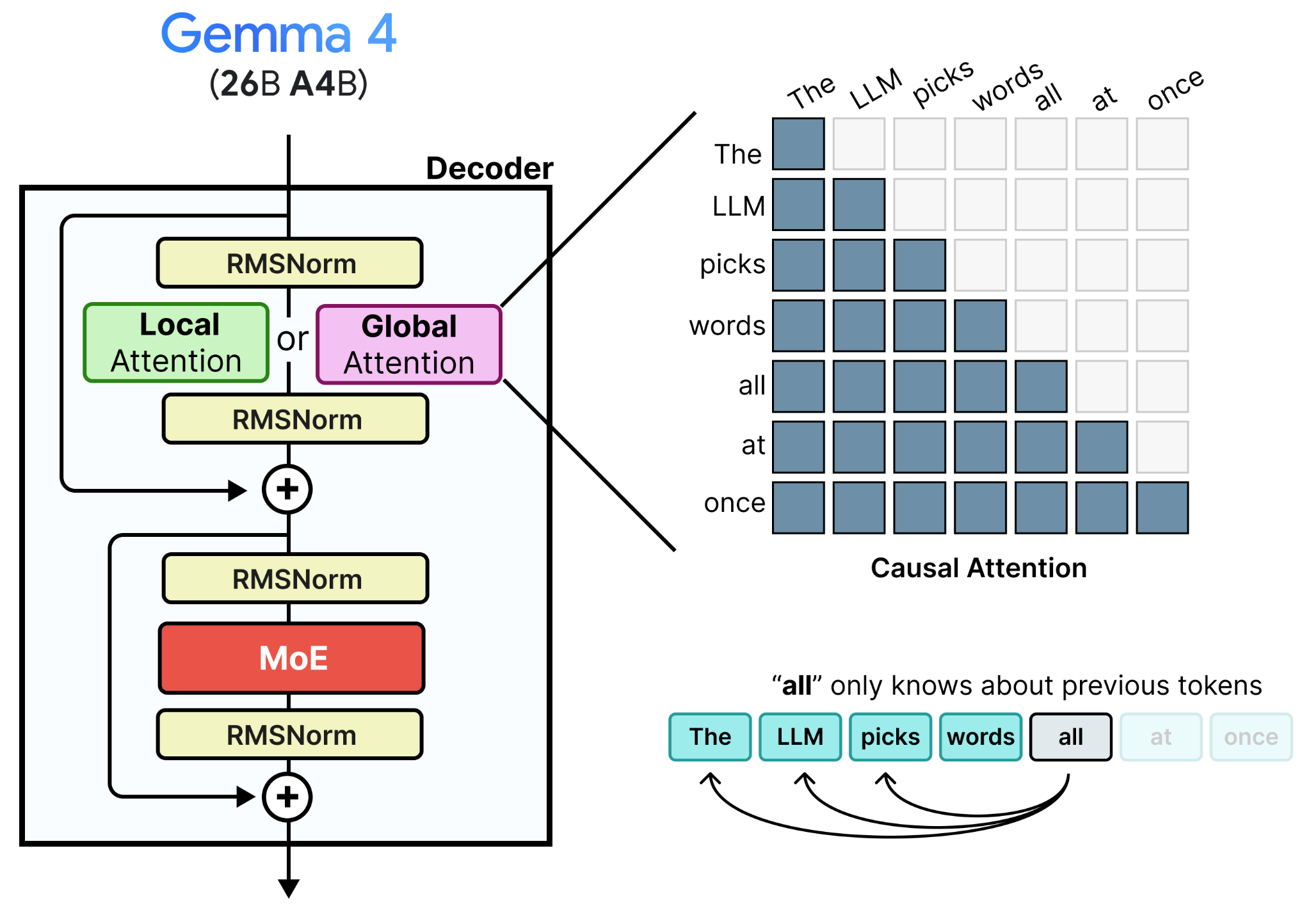
Gemma 4 26B A4B, as covered in A Visual Guide to Gemma 4, is a Mixture of Experts (MoE) model that already went through extensive training and has great performance. There is one problem though…
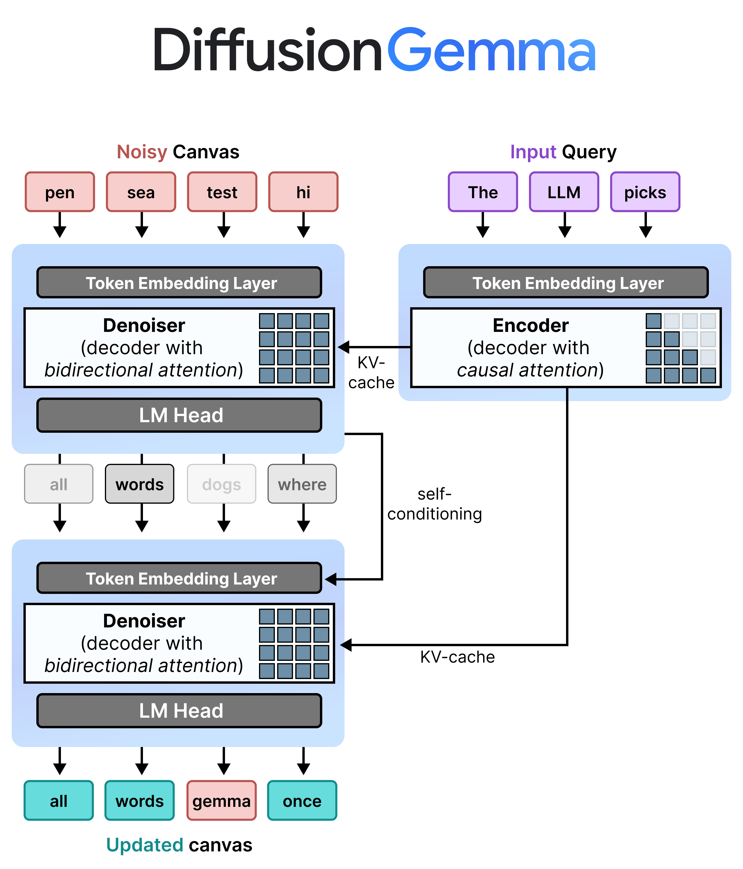
Gemma 4 26B A4B is a decoder-only model and meant to generate text one by one whilst diffusion generally needs an encoder and a denoiser. This is where an elegant solution comes in, the Encoder-Denoiser patch!
This patch is a way to convert a single decoder-only model into a:
Encoder – Used for “understanding” the query
Denoiser – Used for denoising the canvas
It does so by having a single model (Gemma 4 26B A4B) dynamically switch between a denoiser mode and an encoder mode.
Denoiser Mode - Act like an Encoder
To convert a decoder-only model (Gemma 4 26B A4B) into a denoiser, we can make use of something it is not directly using when generating tokens, namely the logits of all tokens!
Specifically, an autoregressive LLM first converts the text into token embeddings (a set of 1-dimensional numerical values). As those token embeddings flow through the LLM, they get processed and updated continuously. This is often referred to as the hidden states of the model. The final hidden states are projected to logits which represent a confidence score for each word in its vocabulary. This means that for each token in the input, a set of confidence scores are generated. However, only logits of the last hidden state are used to choose the predicted token. All other logits are essentially thrown away!
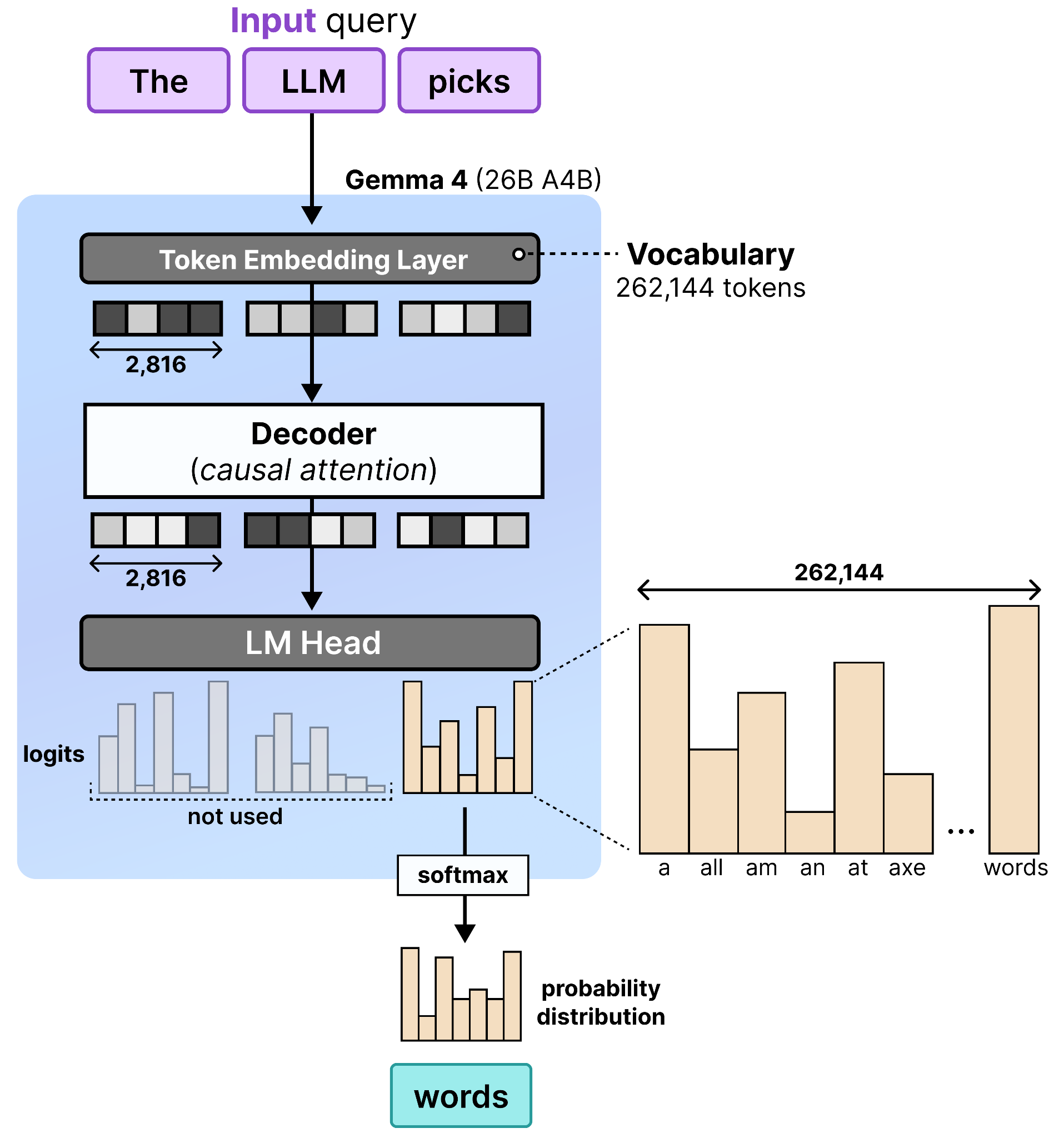
This “throwing away of logits” is not necessarily a bad thing considering the logits of the final token contains all information about the previous tokens. The reason why we only use the final is because each token in a sequence can only attend to (“see”) to the tokens before it. So the hidden state of the final token is an aggregation of the entire sequence, which you need to predict the next word.
This leads to an interesting idea. What if we were to replace two things:
The input sequence of tokens with a canvas
The causal attention with bidirectional attention
Since the model should work as a denoiser, we expect the input tokens to be a noisy canvas instead. With causal attention, however, that would still mean that the logits at each position only attend to information that came before it. Since we want to generate a sequence of tokens all at once, we do not want a given token to be unaware of the tokens that come after it, noisy or otherwise. We instead have to replace causal attention with bidirectional attention. This makes it so that a token can attend to all other tokens in the sequence, regardless of their relative position.
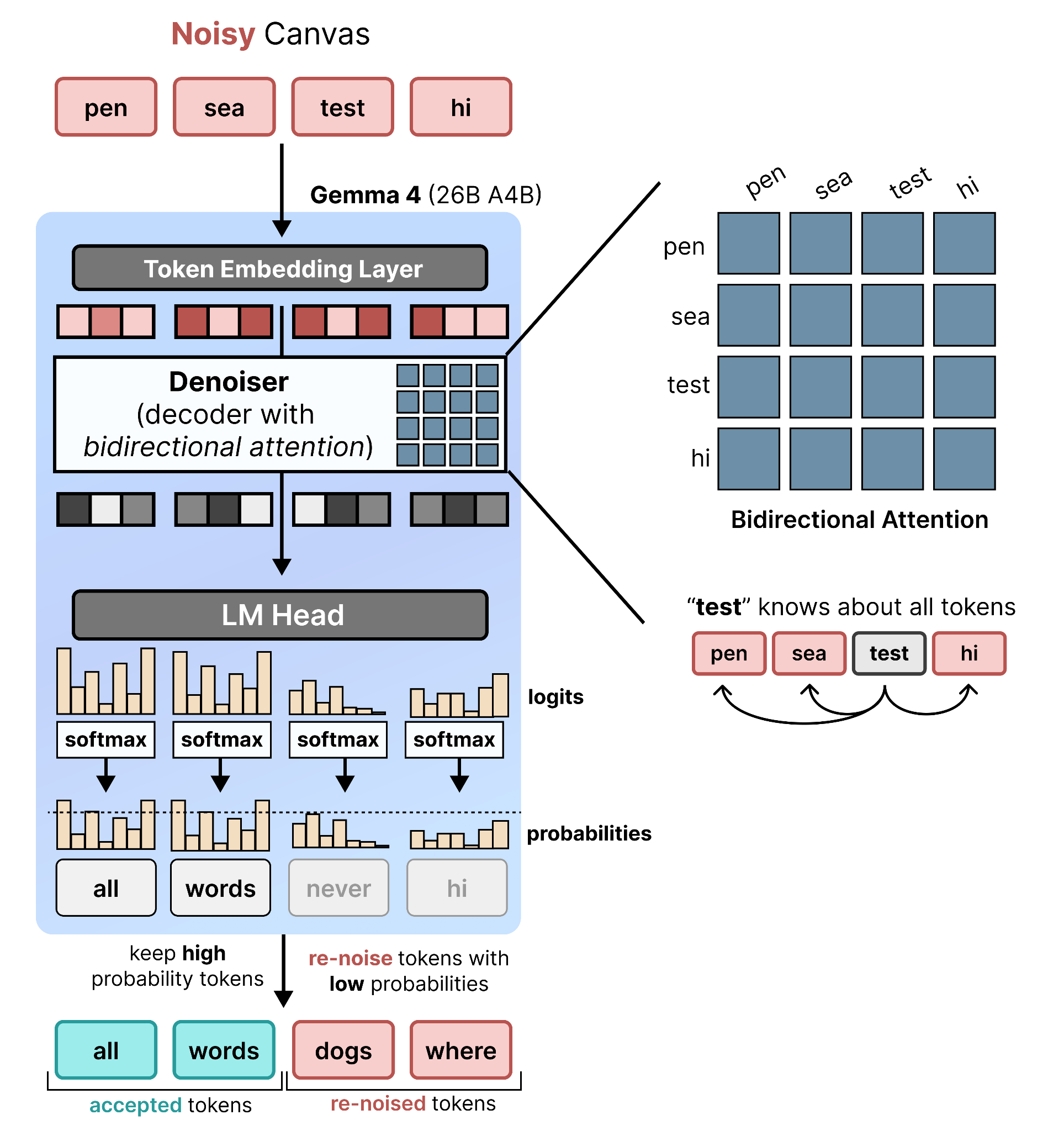
With bidirectional attention, we can now use the logits of all tokens in the input noisy canvas as all tokens attend to one another. For each position in the noisy canvas, the best matching token is selected. If that token has a high probability, it is accepted but if it still has a low probability then it is re-noised and replaced with a different random token.
When you replace an attention mechanism, it doesn’t just work out of the box. Gemma 4 26B A4B has been trained with causal attention, so it will get confused if it can suddenly use bidirectional attention. That is something you will have to train, but more on that later.
With a noisy canvas as input and bidirectional attention, we can use Gemma 4 26B A4B as the denoiser iteratively updating a canvas. However, without an input query, there is no way for the model to know how to fill in the canvas. That’s where the encoder comes in.
Encoder Mode - Acts like a Decoder
The encoder mode of Gemma 4 26B A4B, like the encoder in image diffusion, is meant for processing the input query and providing context and guidance to the denoiser. Normally, you would use an encoder (LLM with bidirectional attention) to process the input. However, Gemma 4 26B A4B was trained with causal attention and if we were to replace it again, that would be rather costly. Instead, we can use Gemma 4 26B A4B as is to perform the query processing. This Gemma 4 26B A4B model isn’t used natively but fine-tuned to support the different tasks of denoising and encoding.
In this process, we do not use the LM Head since we are not generating tokens, but token representations instead. These representations generally come in two ways, either the hidden states or the KV cache.
However, using the hidden states would require additional cross-attention which is yet another patch. Since the encoder mode and decoder mode share the exact same model, with different attention mechanisms, DiffusionGemma shares the KV cache instead between the encoder mode and the decoder mode.
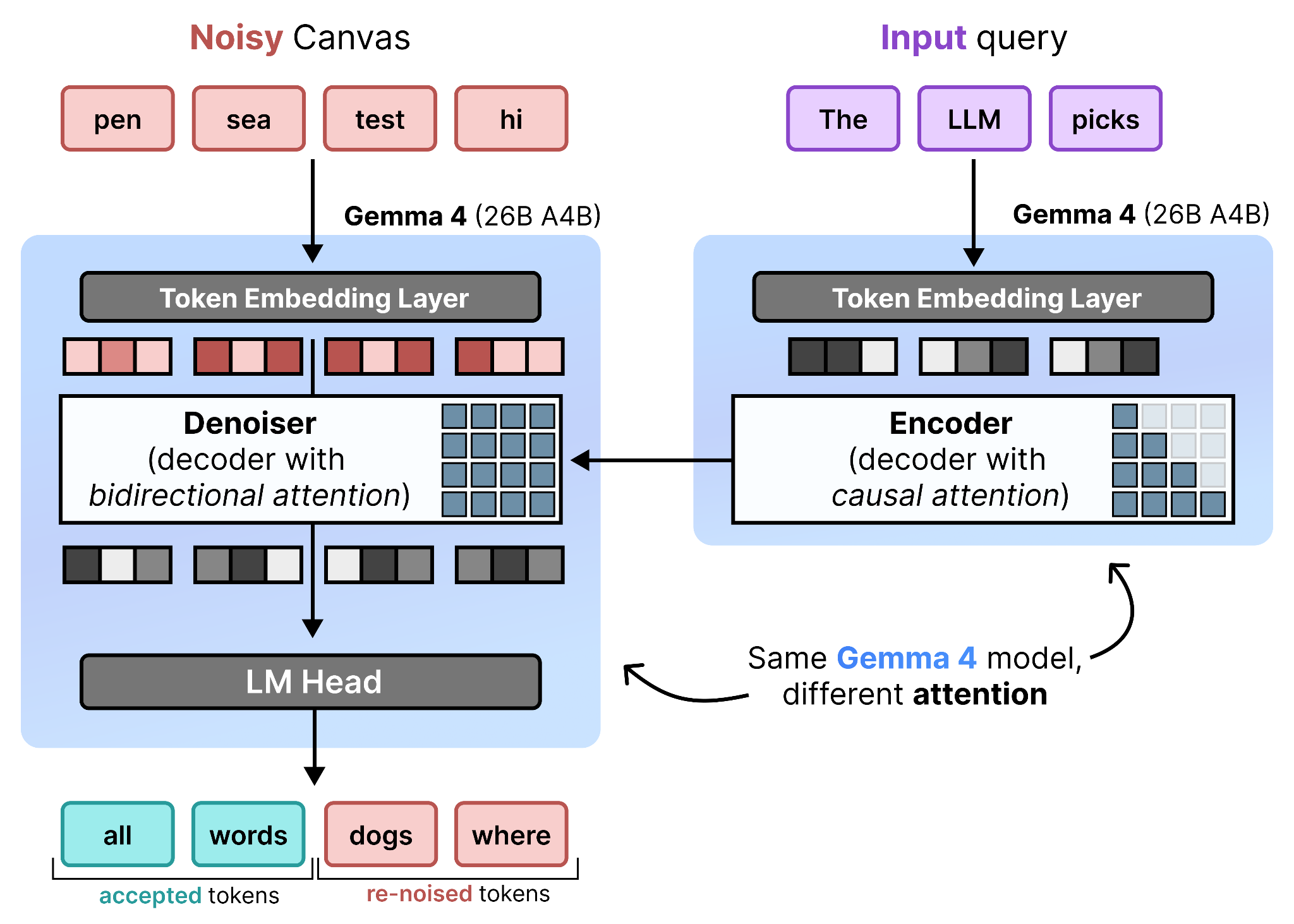
Another reason is that even though the Encoder is a Decoder model with causal attention, it can still generate great representations of the input query. As such, these KV-cache representations are shared with the Denoiser (Gemma 4 26B A4B with bidirectional attention) so that it understands what the user actually wants it to generate. The KV-cache is not updated throughout the denoising steps of the Denoiser.
Inference of DiffusionGemma
A big part of diffusion models is how they handle inference. Specifically, the canvas is not generated in a single step but iteratively updated. This results in several questions we have yet to answer:
How does the model know about predictions it made in the previous step?
How do you generate a sequence that is larger than the canvas?
How many denoising steps does the denoiser use?
Self-Conditioning
The first question that we answer is “How does the model know about predictions it made in the previous step?”.
The answer, fortunately, is quite straightforward. After the denoiser has run a single step it can use the probabilities that it generated and pass it along to the second step. This gives the model information about what it intended to do the previous turn and where it came from.
In practice, it does so by multiplying the probabilities after the softmax with the embeddings of all tokens, also called the embedding matrix or embedding table. This multiplication results in one embedding per position in the canvas that represents this probability distribution. As such, it puts more weight on the embeddings of more probable tokens. They are then passed to a small feedforward neural network (FFNN) and added to the token embeddings in the next step.
This essentially gives it a memory of what it attempted to do in the previous step and how confident it was when predicting certain positions.
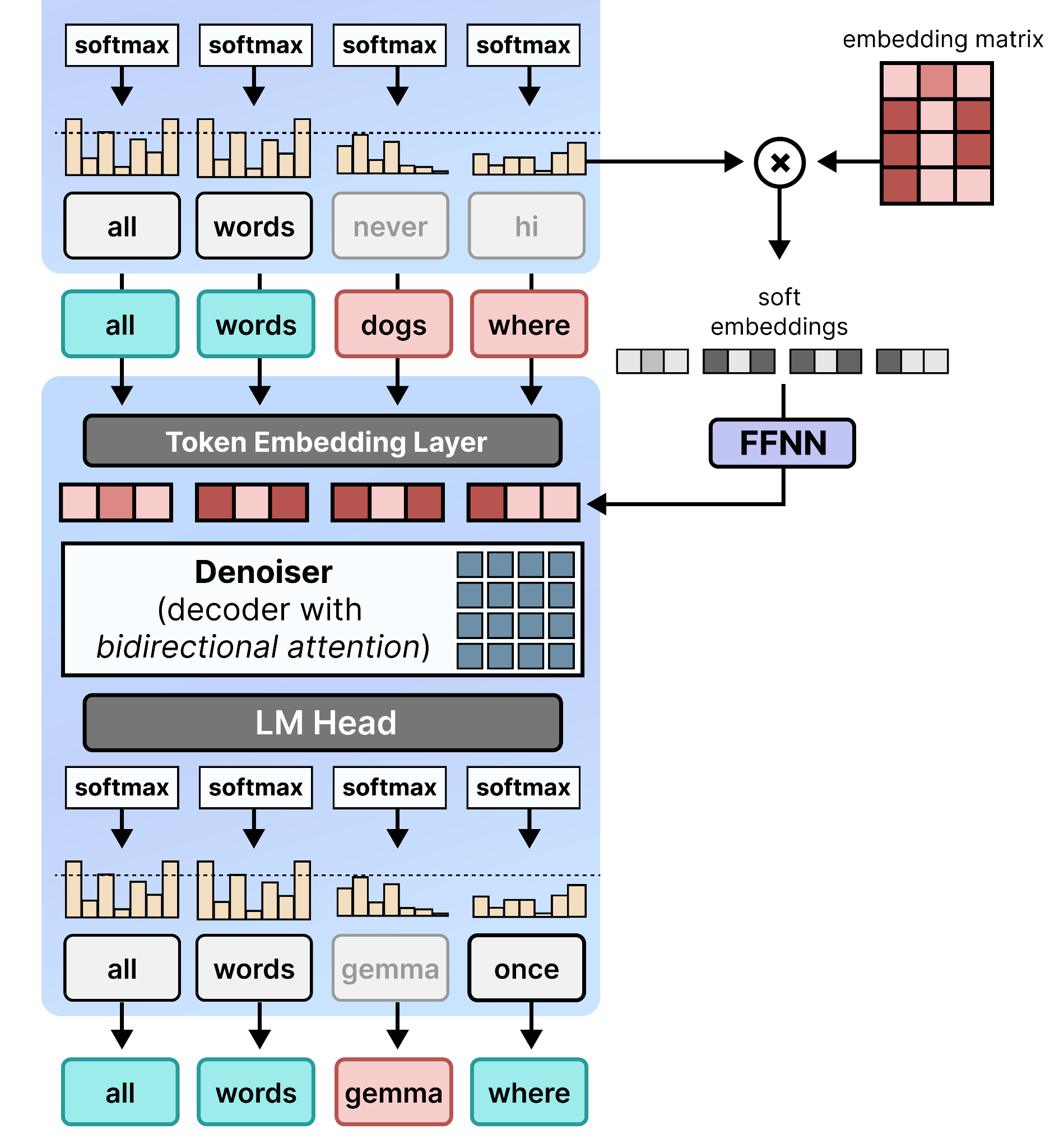
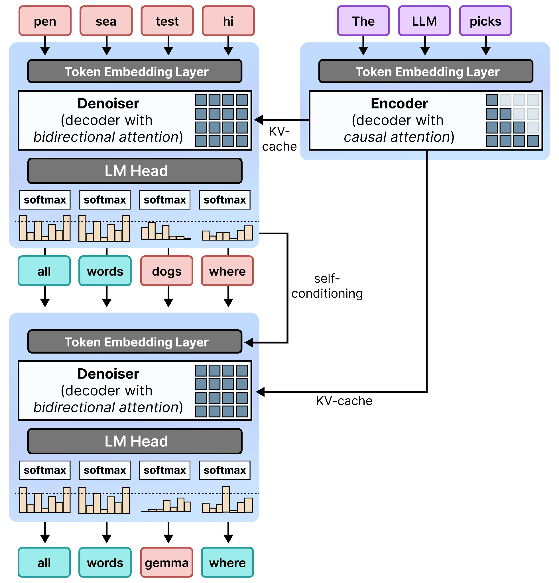
When you put everything together, the second step is exactly the same as the first step and re-uses the KV-cache of the encoder. This self-conditioning on the previous step can be seen as a skip-step where information is propagated to the next step so it can continue the process with more context.
We now have the full architectural overview of DiffusionGemma:
Multi-Canvas Sampling (Block Diffusion)
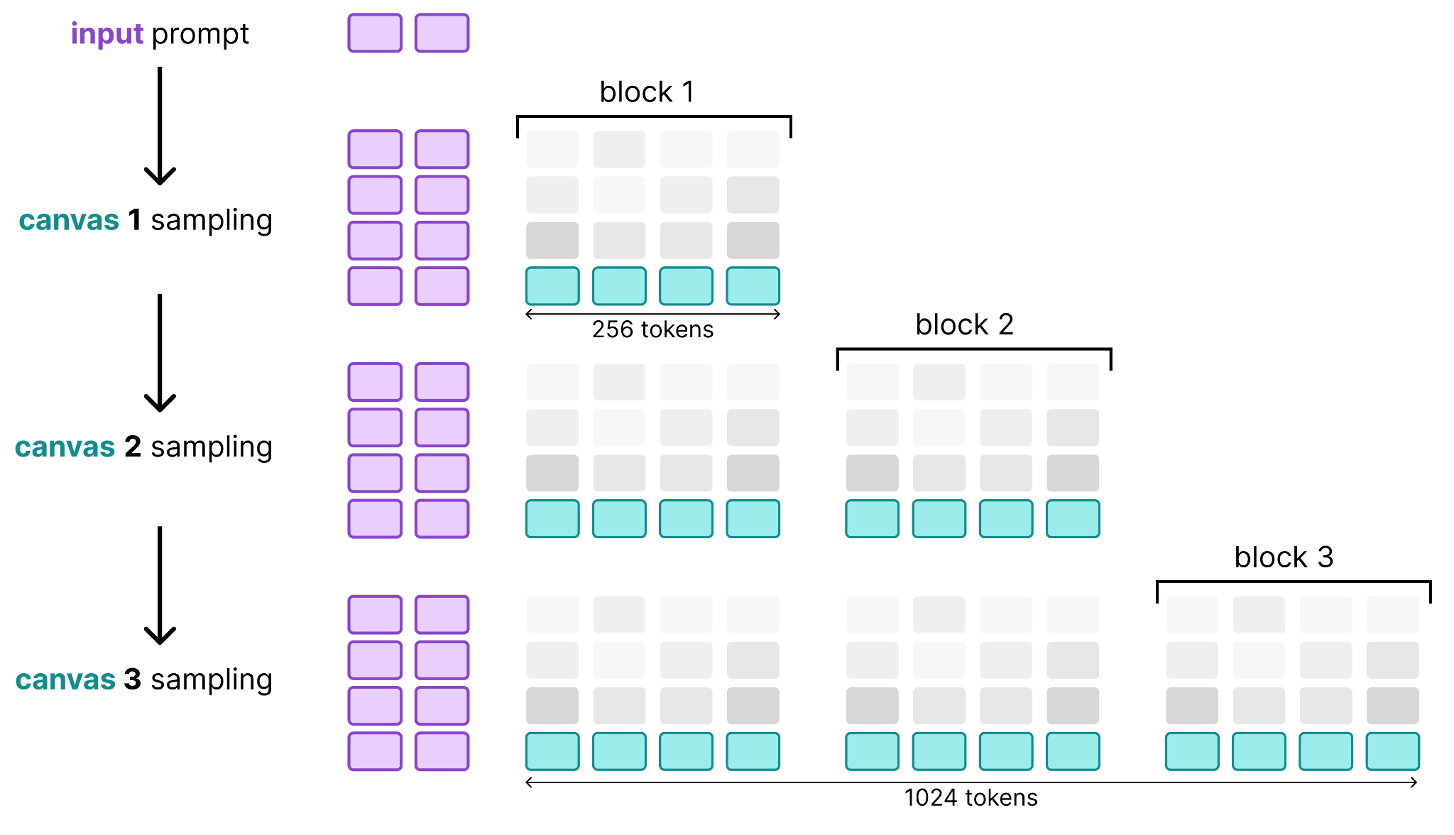
The second question that we need to answer is “How do you generate a sequence that is larger than the canvas?”.
The canvas in DiffusionGemma has a size of 256 tokens, which isn’t all that big! Fortunately, we can mix and match diffusion with autoregression together to expand the number of tokens that are generated.
Specifically, we first generate the 256 tokens using DiffusionGemma as we explored thus far. Those 256 tokens only need to be passed through the encoder once to generate the KV cache after which the denoiser takes a number of steps to fill up this canvas. When it is finished, the prompt is updated with the new 256 tokens and added to the input sequence of the encoder to extend the KV cache. The denoiser then continues to create another sequence of 256. This process continues until the denoiser generates a stop token.
As such, the canvases are generated using diffusion but are stitched together sequentially. This means that we are alternating diffusion with autoregression!
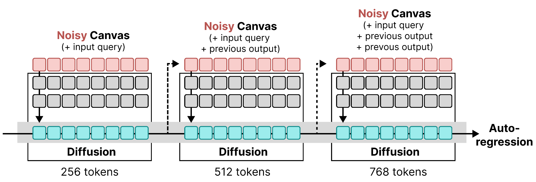
Looking back at what at the figures we used to compare diffusion with autoregression, they are now combined into a process where each diffusion output is appended together in an autoregressive way:
A big part of what makes this possible is that the KV cache for the encoder is calculated using causal attention. Since each token only attends to what came before it, only the KV cache needs to be calculated for the canvases that are added in each “autoregressive step”. The result is a relatively cheap operation since we can continuously update the KV cache rather than having to recalculate it.
A big part of what makes this possible is that the KV cache for the encoder only needs to be calculated at the start of every “autoregressive step”. During a “diffusion step”, the KV cache is reused and does not need to be recalculated since no new tokens are added until the end of diffusion.
The Scheduler
The scheduler in image Diffusion controls how much noise to remove at each denoising step and how many steps to take. In DiffusionGemma, it is a collection of techniques that together decide how the step-based process of denoising works. It “schedules” the denoising process and doesn’t decide directly which tokens to reject or accept. In contrast to image Diffusion, the scheduler in DiffusionGemma consists of three separate components working together.
First, the step count. This decides how many maximum denoising steps there are. More steps generally means higher quality output but slower generation.
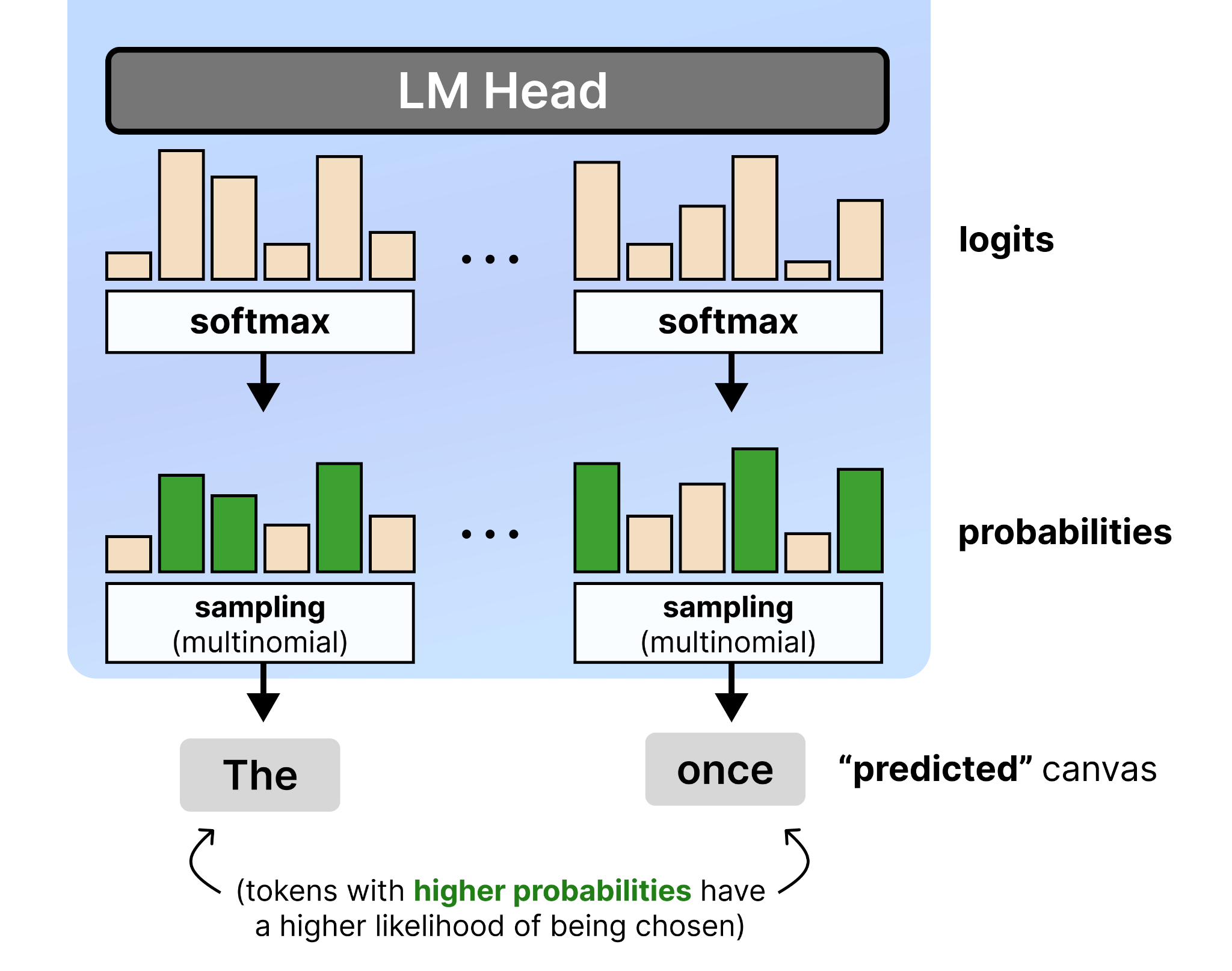
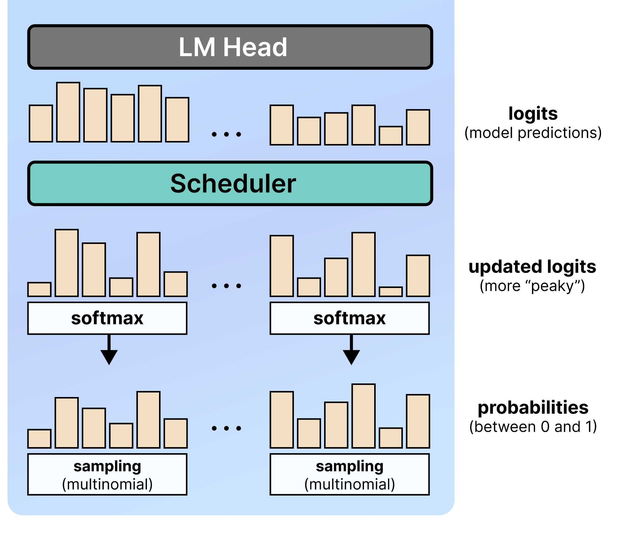
Second, the logits scheduler. After the model generates its raw logits, they are converted to probabilities via softmax. From those probabilities, it is now always the most probable token that is selected. It selects the token based on a multinomial distribution. This means that tokens with high probability have a higher chance of being selected and vice versa.
There is a problem though with the generated logits, namely that they tend to be more uncertain. The reason for this is that at each step in the denoising process, there are noisy tokens in the canvas which might hurt the predictability (and therefore the logits) of each position.
The logits scheduler makes sure that the model’s predictions (the logits) are more decisive. It does so by dividing the logits by a temperature value. This value is the same as you see in Autoregressive LLMs.
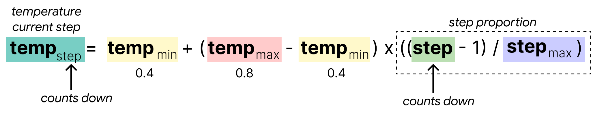
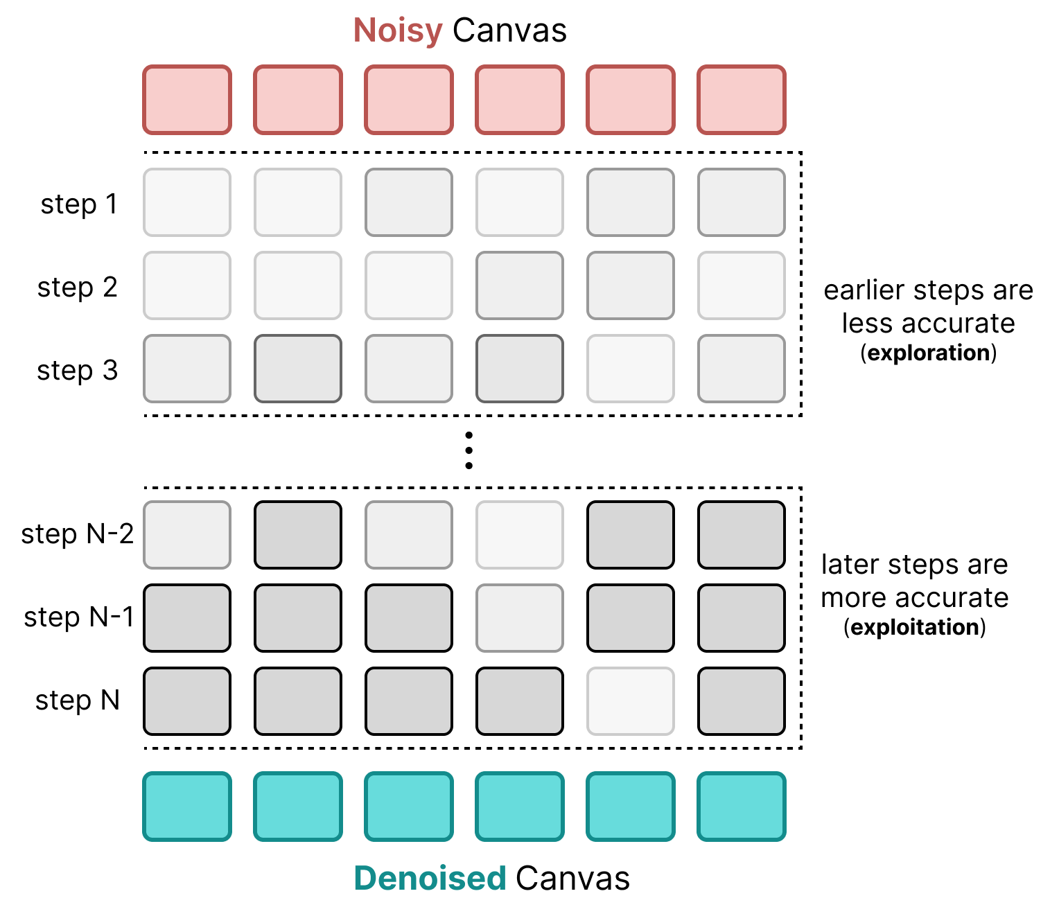
Note that the steps count down instead to make sure that at each denoising step has a lower temperature:
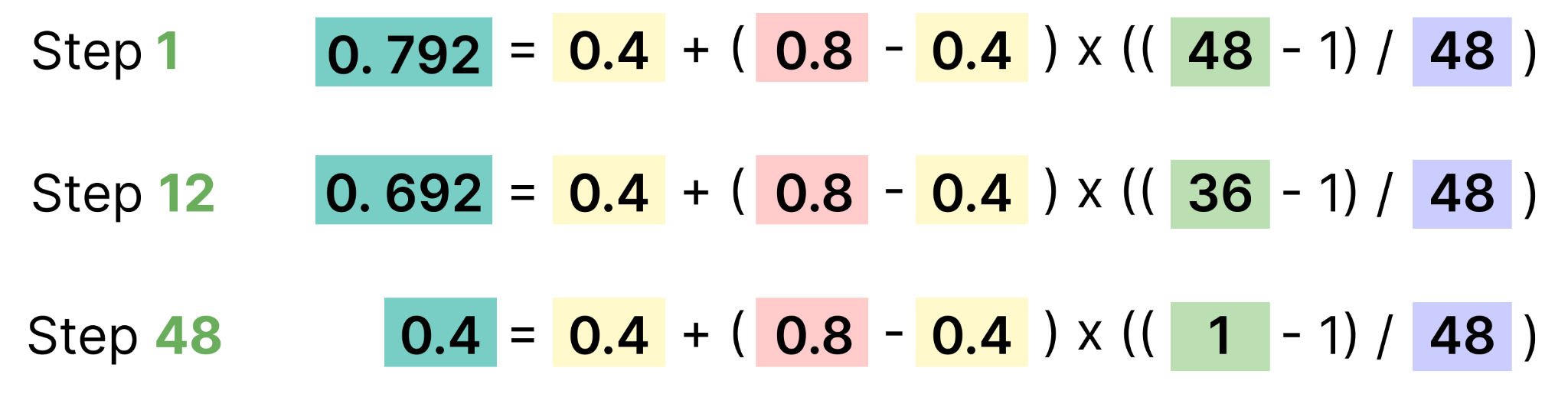
Dividing the logits by the temperature at each step helps make the logits distribution more distinct or “peaky“. Since the early canvas is mostly noise, sharpening predictions will have little meaning anyway. Only at later steps does the model have a cleaner canvas and we can sharpen the predictions.
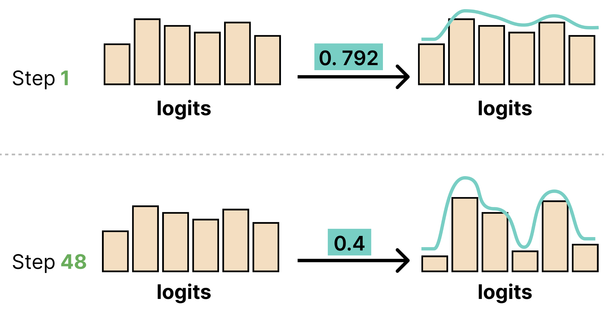
This means that in early steps, the model will explore a bit more and not just focus on the most probable tokens. Whereas in later steps, the model will explore less and focus more on the most probable tokens. It enforces a balance between exploration (early steps) and exploitation (later steps).
As such, we can see the earlier steps as a bit more “noisy” with respect to token distributions compared to later steps.
Third, adaptive stopping. Although the step count already defines the maximum number of steps the denoising process can take, the model might converge early on. For that, there is the adaptive stopping mechanism. At every step, it checks:
Stability – Have the highest-probability token predictions been identical for the last N steps?
Confidence – How confident is the model across all tokens in the canvas?
In the configuration of DiffusionGemma, the confidence threshold is 0.005 and the stability threshold is 1. Confidence is measured by how spread out the model’s predictions are, which is referred to as entropy. In a given canvas position, if a token’s probability is quite high (e.g., 95% to “LLM”) it is confident and the entropy is low. This means that if the model is confident across most token positions and the predicted tokens are the same as in the previous step, then the model will stop generating regardless of how many steps it has left.
The Entropy Bounded Sampler
In image diffusion, the sampler controls how to combine the model’s prediction with the current noisy image to produce the next, slightly-less-noisy image. In DiffusionGemma, it controls the amount of noise during the denoising process. Each sampler consists of three components:
Canvas initialization – How the noisy canvas is created.
Token acceptance – Which of the predicted tokens to keep and reject
Token re-noising – How rejected tokens are re-noised
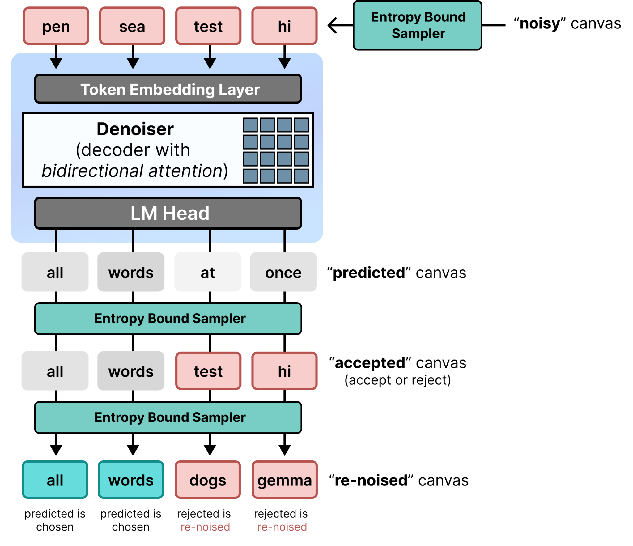
As a default, the sampler used is the Entropy Bounded Sampler.
Canvas Initialization
The canvas is created with random tokens (drawn uniformly) which is essentially the same as starting from pure noise in image diffusion.
Token Acceptance
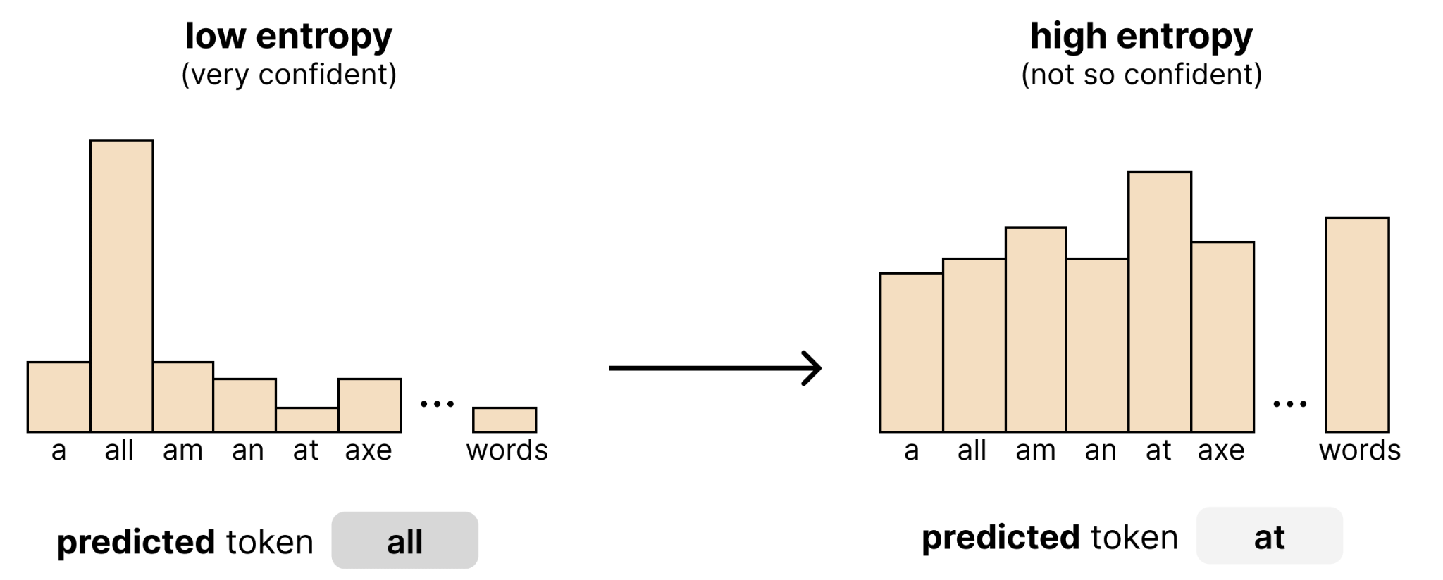
The Entropy Bounded Sampler decides which tokens to keep based on how confident the model is about each one. To measure that confidence, it uses entropy which defines how spread out a probability distribution is. Remember that for each position in the canvas, the model creates a probability distribution. If that distribution leans heavily towards a single token, then it is quite confidence and the entropy will be low. If, however, the distribution is equally distributed (it doesn’t know which token to choose) the entropy will be high.
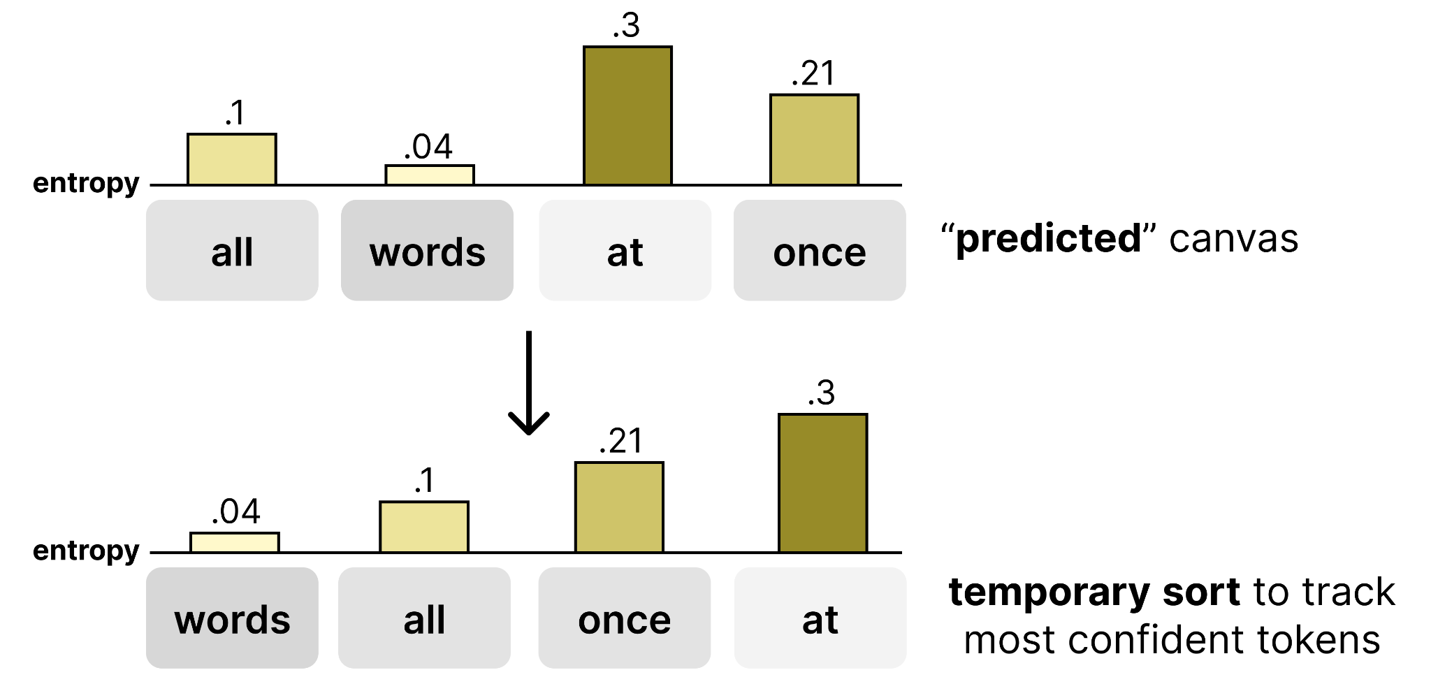
The sampler calculates the entropy value for each position in the canvas. Then, it sorts them from lowest entropy (most confident) to highest entropy (least confident). Therefore, this token list starts from the model’s most confident prediction and the sampler will go through one by one to check whether it can be accepted.
The acceptance criterion is based on the following formula:
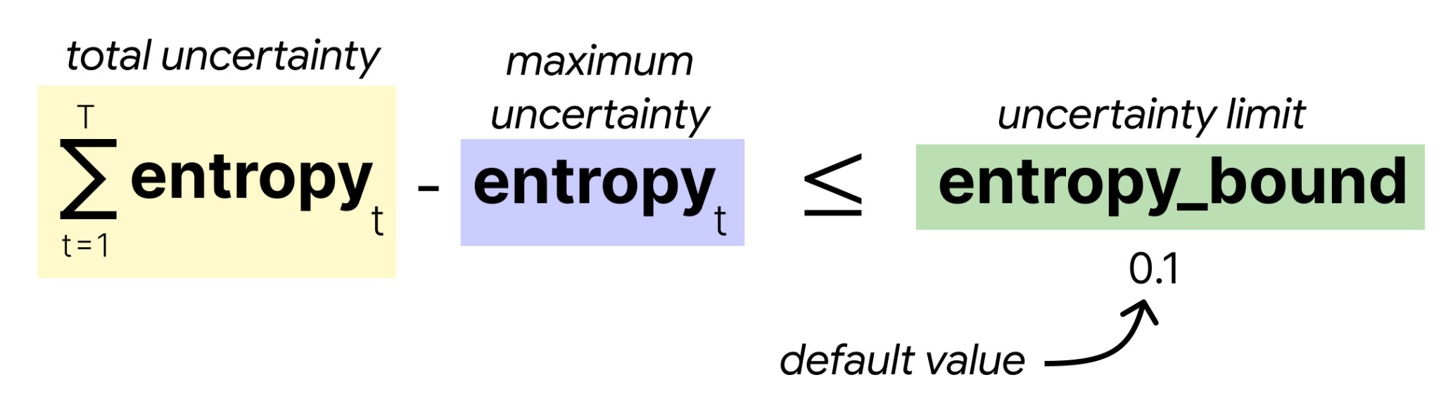
Starting with the canvas position where the model is most confident, the sampler checks whether the sum of entropies seen thus far (minus the maximum entropy) exceeds the limit you set beforehand. If it does, then the model is not confident enough and it will be rejected. If it does not exceed the limit, the model is confident enough and we continue with the next most confident canvas position.
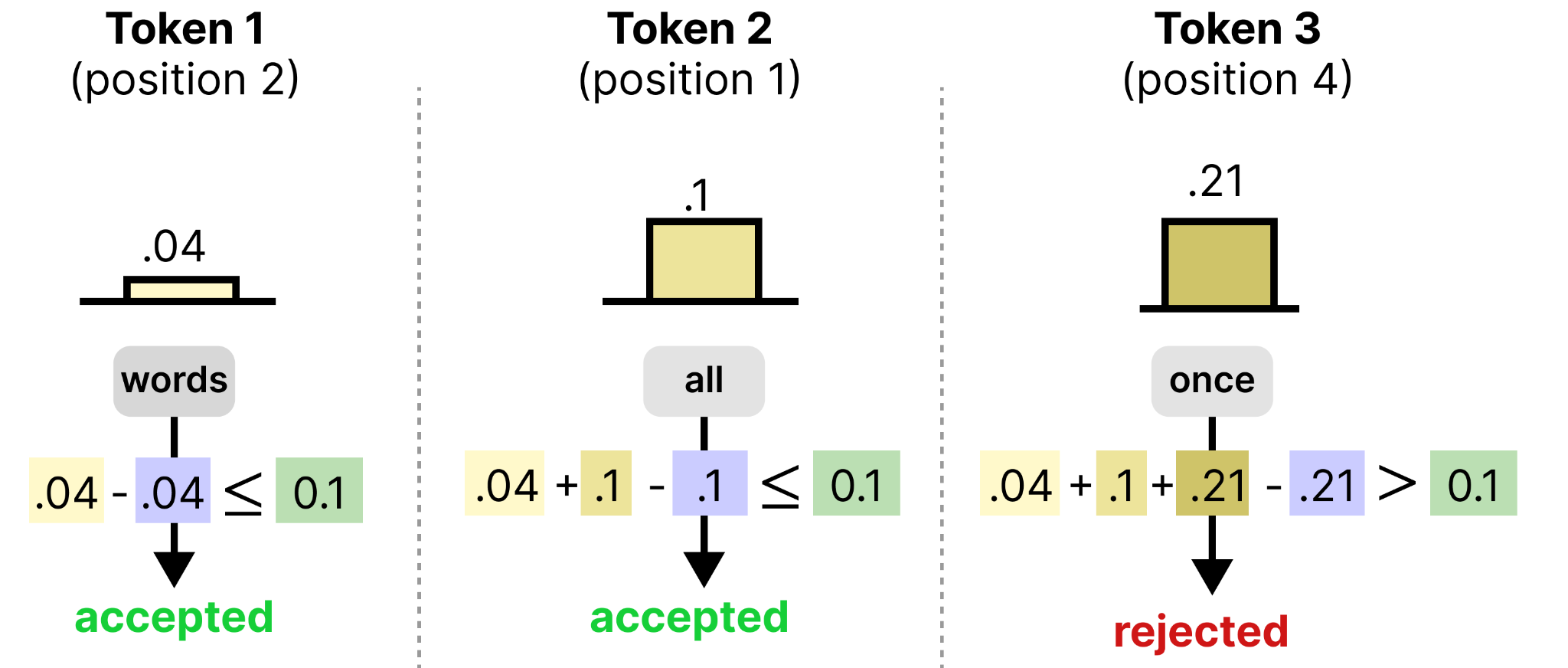
As such, the sampler only accepts a group of tokens when they are each individually confident and as a whole do not exceed the limit. This allows the model to focus more on accepting tokens that it is quite sure are correct, regardless of what the other token positions will be.
Token Re-noising
Re-noising the canvas in the Entropy Bounded Sampler is quite straightforward, all rejected tokens are re-noised! That doesn’t mean though that the accepted tokens will always remain in place. In next denoising steps, the model may decide to give it a lower probability after generating updated context.
Conclusion
What a ride… diffusion in text!
It’s hard to see here, but I actually had to hold myself back from creating 40 additional images and in-depth content.
With that, I hoped you enjoyed this in-depth explainer and that gave you a sense of intuition when thinking about this model. There is still so much to discover about this model and how diffusion works in DiffusionGemma. Compared to text generation, there are new things you can tinker with like building your own samplers!
A very special thank you to the people that gave feedback on this visual guide: Nate Keating, Jean Tarbouriech, Bobak Shahriari, Brendan O’Donoghue, João Gabriel Oliveira, Omar Sanseviero, and as always anyone else I might have forgotten ;)
When I saw that DiffusionGemma was released the first thing I googled was "Visual Guide to DiffusionGemma" and you didn't disappoint 🤭
Hi Maarten, incredible guide! The decisions made throughout this paper are genuinely inspiring. I wanted to ask more details on switching between causal attention to bidirectional attention for the Gemma 4 model as you had mentioned "more on this later" earlier. Would love to know how you differently you expect it to perform if it was trained bidirectionally from scratch as well.